In this experiment, we will start by becoming familiar with the characteristics of the Geiger-Müller (GM) tube, a type of ionization detector. Then we will use the GM tube to perform a simple counting experiments for the purpose of studying some of the techniques of statistical analysis. Finally, we will measure the half-life of an excited state of the \( ^{137}\mathrm{Ba} \) nucleus.

Details about Geiger-Müller tubes

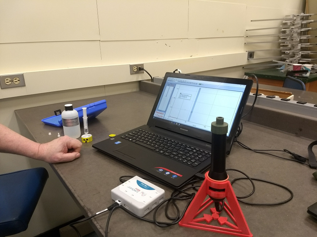
In our experiment we will use a Vernier Radiation Monitor which uses an LND 712 Geiger-Müller tube operated at a fixed 500 Volts. The computer interface provides the DC power (using a dc-dc upconverter) and plays the role of the oscilloscope to record counts. There is a discriminator function which decides whether a pulse is sufficiently large to count. Since the G-M tube is operated in the G-M range ¹, no energy information is preserved.

Open the Logger Pro program to access the counting software. The LoggerPro program should recognize a "Radiation Monitor". Use the "Data" menu to change parameters when you take data.

1. Measure the room background count rate. Record the number of counts N per 10 sec interval for several intervals. Plot the number of counts per 10 sec interval as the abscissa and the number of times that number of counts occurred as the ordinate of a graph ¹.
2. Determine the mean number of counts \(\langle N \rangle \) and the standard deviation \( \sigma\). The result should approximate the “Poisson” distribution, for which the probability P for observing N counts in a given time interval is given by

$$ P(N)=\frac{\langle N \rangle^{N}e^{-\langle N \rangle}}{N!}\, , \, \sigma=\sqrt{\langle N \rangle} $$

Compare your graph with this expression.

Now take a \(^{137}Cs\) sealed source. This sample has a thin window on one side that allows both the beta radiation (coming from the \(^{137}Cs\) decay) and the gammas (coming from the \(^{137}Ba^*\) decay) . What do you think the actual rate of particles generated from the two decays should be? When you measure the count rates from the two sides of the source how do they differ. Why do you think this is?

Put convenient materials (paper, thin metal, plastic) between the souce and detector with both "blue" and "yellow" sides facing the G-M tube. Summarize your observations.

Move the \(^{137}Cs\) sealed source away from the detector. Does the count rate change? How would you expect the count rate to change with distance and what other factors would affect this rate?

1. Set the source a distance from the detector so that the count rate is \(\approx 10\) counts per 10 sec interval.
2. Repeat the procedure of Measurement 1 and make a histogram of the results.
3. Determine the mean number of counts \(\langle N \rangle \) and the standard deviation \( \sigma\). The result should approximate a “Gaussian” distribution, for which the probability P for observing N counts in a given time interval is given by

$$ P(N) = \frac{1}{{\sigma \sqrt {2\pi } }}exp(-\frac{1}{2}\frac{(N-\mu)^2}{\sigma^2}) \, , \, \mu = \langle N \rangle $$

Compare your graph with this expression.

We will now measure the half-life of an excited state of the \(^{137}Ba\) nucleus ². Samples are prepared from a radioactive isotope of \(^{137}Cs\) using a chemical that only dissolves Ba ³. The lab staff or your TA will prepare this sample for you.

This isotope has too many neutrons to be stable; it decays by \(\beta\)-decay into \(^{137}Ba^{*}\). This daughter nucleus is produced in an excited state, indicated by the asterisk \(^{*}\). The excited state subsequently decays into the ground state of \(^{137}Ba\) with a half-life of the excited state of 2.6 min. The decay of the excited state is detected by measuring the emitted \(\gamma\)-rays of 0.66 MeV. This energy corresponds exactly to the energy difference between the excited state in \(^{137}Ba^{*}\) and the ground state.

The \(\gamma\)-ray emission rate \(R(t)=-\frac{dN(t)}{dt}\), where \(N(t)\) is the number of \(^{137}Ba^{*} \) nuclei present at time \(t\). The emission rate is proportional to \(N(t)\):

$$ \frac{dN(t)}{dt}=-\lambda N(t) $$

where the proportionality factor \( \lambda \) is defined as the decay constant. Integration of the above expression leads to

$$ N=N_{0}\exp(-\lambda t) $$

where \(N_{0}\) is the number of excited nuclei present at t=0. The half-life \(t_{1⁄2}\) is defined as the time it takes for the activity to be reduced by half; thus, at \(t=t_{1⁄2}\), \( N=\frac{N_{0}}{2}\). Derive the relationship between \(\lambda\) and \(t_{1⁄2}\) . Show that at any time \( t+t_{1⁄2}\) , there will remain only one-half of the excited nuclei that were present at time \(t\)!

1. Use a freshly prepared (!) sample of \(^{137}Ba^{*}\) , place it under the Geiger counter, and measure the decay rate \(\Delta N \) in some suitable time interval \(\Delta t\) as a function of the elapsed time. Continue until the count rate is comparable with the background rate over the same time interval.
2. Correct your data for the background and plot the logarithm of the corrected count rate versus the time \(t\). You should obtain a straight line. Don't forget to put proper error bars on your data points. From the slope of the straight line you can obtain the half-life and the decay constant (including the errors). Compare with the accepted values.