The purpose of this lab is to measure the gravitational acceleration constant \(g\) by studying the projectile motion of an object (motion in 2D). ^{Hoveroverthese}

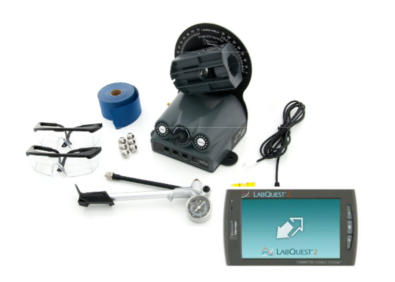
Equipment

• LabQuest 2
• Vernier Projectile Launcher
• Hand pump
• Steel balls and roll of waxed marking paper
• Level and meter stick
• Pairs of safety goggles

Projectile motion is a motion in two dimensions, which can be described as a uniform motion in the horizontal \(x\) direction (constant velocity) and an accelerated motion in the vertical \(y\) direction (acceleration due to the gravitational force).

It can be shown that an object launched horizontally with a velocity \(v_{x0}\) and dropping a height \(h\) has the following relation between its horizontal distance traveled \(x\) and \(v_{x0}\): $$ x=v_{x0}\sqrt{\frac{2h}{g}} $$

Before starting the lab you should derive this equation in your notebook. Please try to do it yourself before coming to class (hint: consider the equation of motion concerning the y displacement as a function of time \(y = y_0 + v_{y0}t − \frac{1}{2}gt^2\) , where at time \(t\), \(y = −h\) ,and \(x = v_{x0}t\).

The launch point in the projectile launcher is \(0.146\) m above the base and \(0.082\) m from the, so an object shot horizontally on to the table falls through a distance \( h=0.146\) m.

Determine experimentally the relationship between horizontal distance and velocity

• Level the launcher
  • Position the launch chamber horizontally by moving the lower knob on the back of the launcher until the bubble of the attached level is in the center between the two vertical lines, secure the lower knob.
  • By using the upper knob (on the back), adjust the position of the angle marking until the zero degree mark is aligned with the center of the launch chamber, secure the knob.
• Connect the hand pump to the launcher (if it is not).
• Connect the launcher to LabQuest2 using one of the digital plugs (above the LabQuest2), select Table (C) from the upper tabs.
• Ensure that the launch angle is set to zero degrees. You will launch the steel ball at seven different velocities. To change the speed of the launch you need to turn the range knob to release the pressure. Turn clockwise for higher pressure (higher initial velocity), turn counter:clockwise for lower pressure (lower initial velocity). Adjust the initial speed to around 5 m/s. Observe the position of the ball when it hits the table after the launching. Tape the waxed marking paper starting a little further than that position (this is to make sure the waxed paper will cover the whole range of the ball at lower velocities).
• Taking measurements:
  The first measurement will be at a speed of around 5m/s.
  • Pump the hand pump.
  • Press collect data (Start) in the LabQuest2 (green arrow).
  • Press and hold the “Arm” button, and press the “Launch” (while pressing the Arm button) to launch the ball.
  • Measure the horizontal distance x at which the ball lands. Remember that you need to add 0.082m to the distance from the edge of the launcher because the launch point is located at that distance from the side of the launcher. Also make sure to note the value of v x0 which corresponds to each x#value.
  • Turn the range knob counter:clockwise (approximately a quarter of a full rotation) and repeat the measurements, do this six more times.

You will now make use of graphical methods to obtain a measurement of the gravitational acceleration constant \(g\). In this lab we will use two approaches to this, plotting both by hand and using a computer.

Making a graph by hand

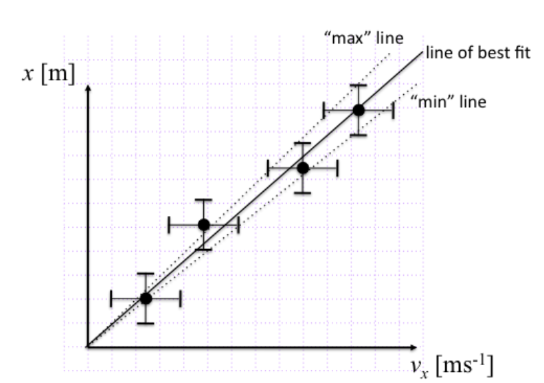
When you make a graph by hand you should use graph paper. Draw and clearly label axes and choose a suitable scale for your data. Represent the error in your values using error bars which extend a distance Δ from your value, where Δ is the absolute error in the quantity. Remember there may be significant errors in both quantities. In some cases the errors in one quantity will be very small relative to the scale of the graph and you may omit them. You need to determine a line of best fit, and measure it's slope. Then you need to draw “max” and “min” lines which correspond to the lines of maximum and minimum slope which fit within the error bars. The slopes of these lines will allow you estimate the error in the slope. In a case such as the present we know the lines should pass through (0,0), this knowledge allows us to put all three lines through that point, substantially reducing the overall uncertainty in the slope.

Making a graph using a computer

While it is important to know how to plot data by hand, in practice physicists will normally use a computer to plot data. You can use the web based plotting tool linked below: Plotting Tools

Calculating the value of the acceleration due to gravity

From your two graphs you now have two different values for the slope and its uncertainty. You should decide which value of the slope and its uncertainty you think is a better representation of the data and use this for your subsequent analysis. We need to calculate the value of the acceleration due to gravity from the slope of our graph. The slope of our graph, which we will refer to as \(k\), is related to \(g\) through equation 2.1, ie.

$$ k=\sqrt{\frac{2h}{g}} $$ We can rewrite this equation as $$ g=\frac{2h}{k^2} $$

Now you need to calculate what the value of \(g\) should be from the value of \(k\) you obtained from the slope of your graph and h=0.146m. Your final task is to estimate the error in our measured value of \(g\) using relations in the Error Analysis Guide.

You should now check whether your measured value of \(g\) is consistent with the accepted value \(g= 9.81 m/s^2\). ¹ Can you think of any ways in which this experiment could be improved to give you a more accurate value for \(g\)?

Guide to Uncertainty Propagation & Error Analysis (Quick Reference)

PHY121/122 Plotting Tool

PHY131/132 Plotting Tool