
Magnetic Force
The purpose of this lab is to explore the relationship among force exerted on a current-carrying wire, magnetic field strength, and the length of the wire. A wire carrying electric current I in a magnetic field B will be subject to a force that is proportional to the length of the wire that is in the magnetic field. If the wire and the magnetic field are perpendicular to each other the force is expressed as $$ \vec{F} = I \vec{l} \times \vec{B} $$ where \(F\) is the magnitude of the force, \(l\) is the length of the wire and \(B\) is the magnitude of the magnetic field. The direction of the force is determined by the right-hand rule. Our goal is to verify that the force is indeed proportional to the current and determine the magnetic field.
NOTE: In this lab you will work with very strong permanent magnets. The magnets are enclosed in the experimental setup so that the magnetic field outside of the setup is not that strong. Nevertheless, working with these magnets can be dangerous. When two of these magnets are close to each other the force can be very large, and the force changes rapidly with the distance. This may cause injury to the person holding the magnets. The magnets may also shatter when they stick together.
- If you have a pacemaker you should not do this lab. You are exempt, and your grade will be determined by the remaining labs.
- Do not hold computers, cellphones or other electronic devices close to the magnets.
- Do not bring magnetic material close to the magnets from the front side. If you do, the plexiglass window may be scratched.
- DO NOT TAKE OUT THE MAGNETS FROM THE EXPERIMENTAL SETUP!
- Current source (DC Power Supply)
- Weights (10 and 20 gram masses)
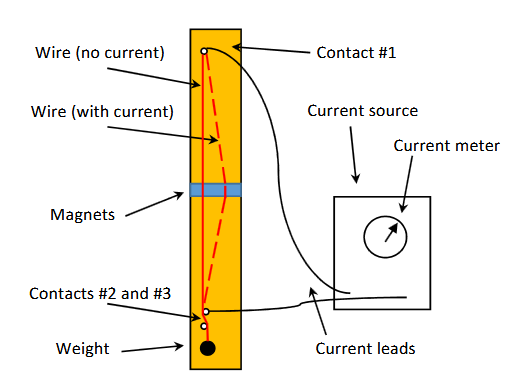
- Magnet and wire assembly (see Figure 1)
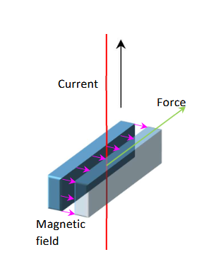
Mag Force Image 2: a current carrying wire in a magnetic field (your directions of B, I and d may vary)
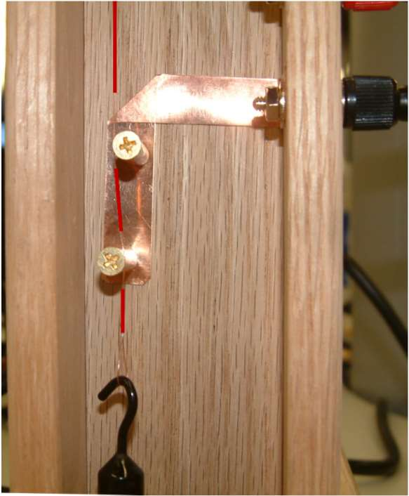
Two very strong magnets with a small gap between them are placed at the middle of a wood board, standing vertically (see Figure 1). A copper wire is attached at the top of the board (contact #1), with a current lead connecting it to the power supply (current source). The wire is threaded in between the magnets, and a weight is attached to the other end (see Figures 1 and 3). The wire is also arranged so that it touches the both of the lower electrical contacts that are also connected by a lead to the current source. Before connecting the power supply, make sure that the wire runs between contacts #2 and #3 at the bottom as shown in Figure 3.
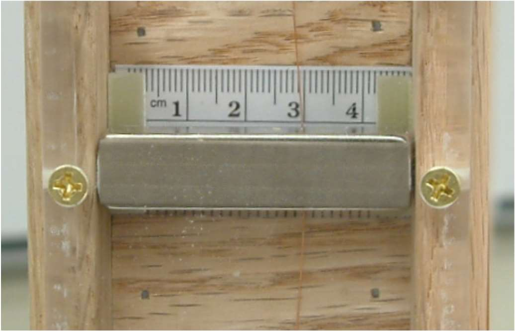
Mag Force Image 3b: wire, magnet and scale
When a current flows through the wire, the magnetic field will exert a force, as illustrated in Figures 2 and 3. This force will pull the wire sideways (when you are facing the board the wire should move to your right side). If we neglect friction and other secondary effects, the position of the wire depends only on the current, the magnetic field, geometrical factors and the weight hanging on the wire.
Know your Power Supply:In this lab we use a power supply that can act as a “voltage source” or a “current source”, depending on the settings and depending on what kind of load is connected to it (a “load” is any electrical circuit that is connected between the red and black terminal).
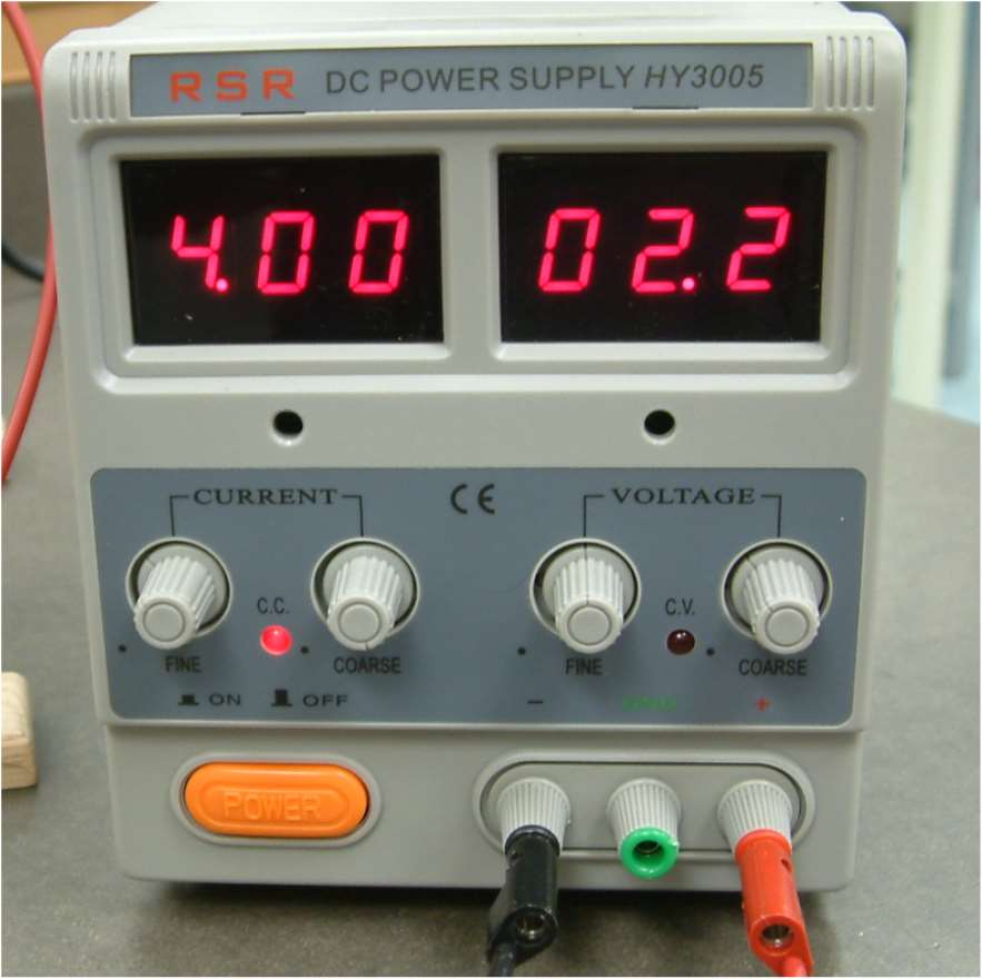
The power supply (Figure 4) has 4 knobs: 2 for current (left side) and 2 for voltage (right side). The “coarse” knobs set the current/voltage in large steps, the “fine” knobs are for precise settings.
Figure 5 illustrates the effect of turning the knobs. The dashed lines are upper limits to the voltage and the current. Within the pink area every voltage and current is possible; voltage and current values outside of the pink area are not possible. Turning the “voltage” knobs adjusts the voltage limit (yellow arrow) and turning the “current” knobs adjusts the current limit (green arrow). If the load has high resistance (blue line) the voltage limit will be in effect and the current limit does not matter. In this case the power supply is a current source (because we can set the current). If the load has low resistance (red line), the current limit will be in effect and the voltage limit does not matter. In this case the power supply is a voltage source (because we can set the voltage). The red light between the knobs tells us which one of the two modes the power supply operates in.
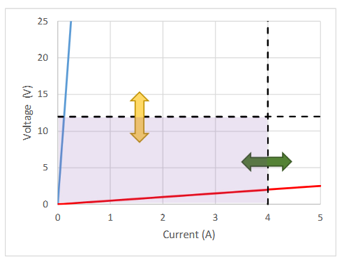
Mag Force Image 5: A map showing the effect of adjusting Voltage or Current
In this lab the resistance of the setup is at most a few ohms. We will work in the current source mode. To set this up follow the next few steps:
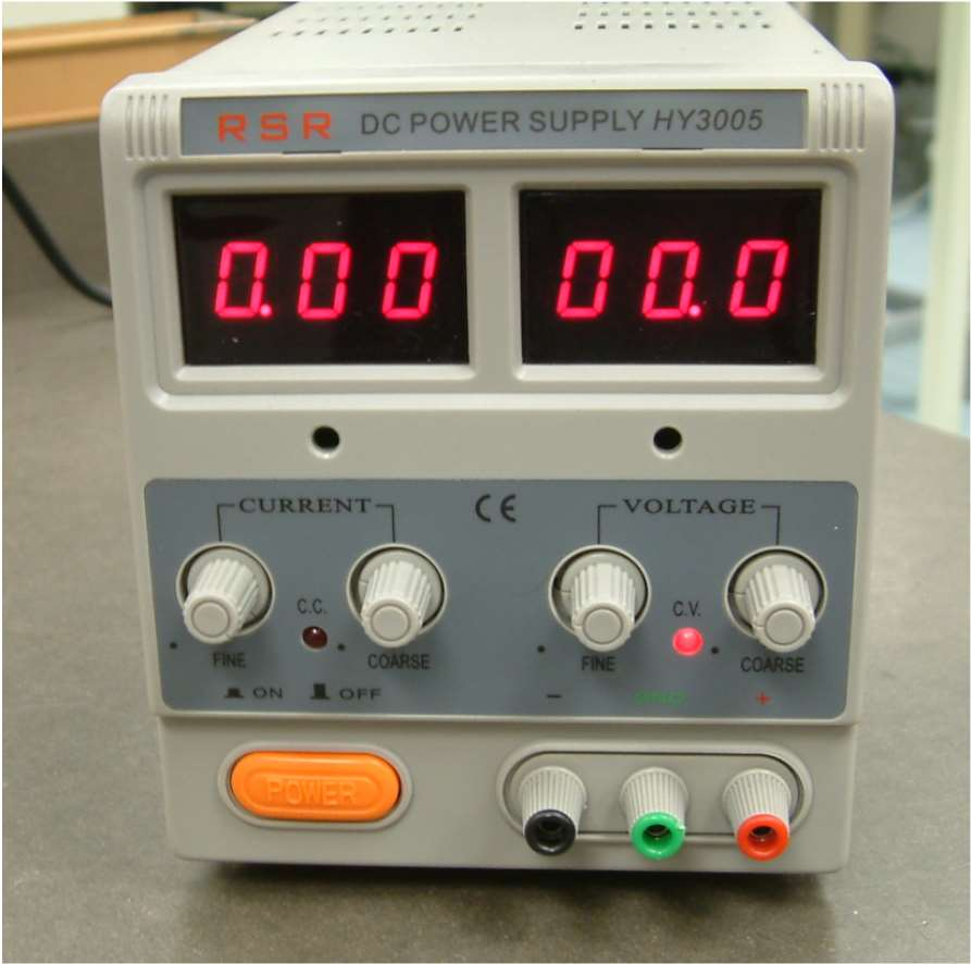
- Before connecting the load (ie. no wired connected to the power supply), turn all knobs fully counter-clockwise. See Figure 6. The supply will be in Current Control.
- Before connecting anything to the source turn the “coarse” current and voltage knobs clockwise just a bit (e.g. quarter turn). The supply will change to Voltage Control.
- Adjust the voltage limit to a value between 5V and 6V.
- Turn the current knobs fully counter-clockwise. You are ready to connect the experimental apparatus.
During the experiment the red light at the current knobs should be on. The voltage should be a few volts at most (see Figure 4 for typical settings with the largest current we will use). If the red light at the voltage light is on, there is an interruption of the electrical circuit, most likely at contacts #2 and #3 (see Figure 3a).
- Make sure that the wood board is approximately vertical and the wire runs between the magnets. Connect a 20g mass to the loop at the lower end of the wire. Thread the wire between the lower electrical contacts, to the left of #2 and to the right of #3 (in an "s", see Fig. 3a).
- Measure the distance \(L\) between contact #1 (the top end of the wire) and contact #2, the upper of the two contacts at the bottom (see Figs. 1 and 3a).
- Switch on the power supply and set it to zero, as described above. Connect the power supply to the measurement setup: red to red and black to black.
- Turn up the current and observe the movement of the wire. Do not apply more than 4.0A, because the wire may melt due to the power dissipated in the wire.
- If the wire does not move or moves in the wrong direction, check you connections.
- Turn down the current to zero. Look at the scale behind the wire and read out the position \(x_0\) in mm. Record it. Increase the current to 0.66A and watch the wire move. Read out and record new the position \(x\).
- Repeat this procedure until the current reaches 4.0A. Take the same set of data in reverse order, starting at high current and going to zero current. At the end read out the position of the wire at zero current and compare it to the value you recorded at the beginning. The two values should agree within the error.
- For uncertainties, note the fluctuation of the current readout and estimate the uncertainty of the current (\(\sigma I\)). If there is no fluctuation, than the current is stable to 3 significant digits and therefore the error in the current is negligible.
- Estimate the uncertainty of the position \(\sigma x\) and the displacement, \( \sigma d\). For example, you may take the error in \(d\) to be ±0.5mm, or if you are more confident in your readouts, take ±0.2mm.
Evaluate the Data
- For each value of current \(I\), calculate the displacement, \(d = x - x_0\)
- When you are calculating the error of \(d\), use $$ ∆d = \sqrt{ (∆x)^2 + (∆x_0)^2} $$ Since the error of \(x\) and \(x_0\) is the same, \( ∆d = √2∆x = 0.7∆x\)
- Plot the displacement \(d\) versus current \(I\) for both data sets . If the current was stable, enter error bars to the displacement only (“y” direction). The data points should be approximately on a straight line.
Answer these questions:
- Q1. According to the graph, what is the relationship between current and the displacement?
- Q2. Look at the slopes for the two measurements (one with 20g mass and the one with 10g mass on the copper wire). How does the slope parameter depend on the weight you applied?
- Q3. Look at the error of the slopes from your two plots. Which one has a larger error? What can be the source of the error in this measurement?
Consider the free body diagram of the wires with the relevant forces (Figure 9), as well as a diagram of geometric displacement (Figure 10). Assume there is no friction and the bending of the wire requires such a small force that we can neglect it:
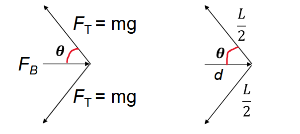
Mag Force Image 10: Relevant lengths assuming \(\theta\) is small
From force balancing (in the small angle approximation) we have the following expression for the displacement of the wire: $$ d= \frac{FL}{4mg} $$ where \(L\) is the distance between the top end of the wire and the upper of the two contacts at the bottom and \(m\) is the mass hanging on the wire. Combined with Eq. (1) we get: $$ d= \frac{BlLI}{4mg} $$ In your plot, \(d\) is on the \(y\)-axis and \(I\) is on the \(x\)-axis. If we fit a line to the data with the usual formula we can identify slope and intercept: $$ Slope = \frac{BlL}{4mg} $$ Ideally, the y-intercept should be zero within uncertainty. The other variables include \(B\) (magnetic field strength in Tesla), \(l\) (length of the wire in the magnetic field, in meters), \(L\) (length of the entire wire between the leads, in meters), \(m\) (hanging mass, kg), and \(g\) (acceleration due to gravity, 9.8023 \( m/s^2\) on Long Island ). Using Eq. (4) we get $$ B = \frac{4Amg}{lL} $$ Remember, \(l\) is the length of the wire that is in the magnetic field, and \(L\) is the full length between the electric contacts. The size of the magnets is 0.50” by 0.50” by 2.00”. Which one of these lengths corresponds to \(l\) ?
Evaluate \(B\)
- Calculate the magnetic field from the measurement when the 20g was used. Use the slope (and uncertainty in slope)from your plot.
- Note: The units of \(slope\) and \(\sigma(slope)\) should be length/current \( = m/Amp\). If you plotted the displacement in units of mm, the values you obtain are in units of mm/Amp, and you need to convert them to m/Amp.
- To evaluate the error of the magnetic field, assume that the weight of the mass is known with such a precision that its error is negligible. Estimate the error of \(L\), \(\sigma L\). Calling the \(slope\) "\(A\)", we get the expression: $$ \sigma B = \sqrt{ ({\frac{\sigma A}{A}})^2 + ({\frac{\sigma l}{l}})^2 + ({\frac{\sigma L}{L}})^2 } $$
- Repeat the calculations with the measurements using the 10g weight.
Questions
Answer these questions:
- Q4. Derive Equation 3, the expression for the displacement of the wire as a function of \(I\) and \(B\).
- Q5. Compare the results using 20 g mass and 10 g mass. Do they agree within the error that you calculated?
- Q6. Compared to the Earth’s magnetic field, how many times stronger is the magnet?
- Q7. Using the right hand rule, draw a diagram showing the direction of the current in the wire, the orientation of the magnetic field between the magnets, and the direction of the force on the wire in the field.