
Faraday's Law

The purpose of this lab is to study the voltage induced across a solenoid coil by the change of the magnetic flux through the coil. You will collect potential versus time data for a magnet moving through a coil and relate the induced emf to changes in the magnetic flux passing through a coil.
- LabQuest 2
- Enameled wire
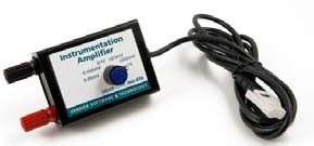
- Vernier instrumentation amplifier
- Neodymium magnet
- Scotch Tape
- Sandpaper
- Pencil
- Sheet of paper
- Record data in this (draft) Google Sheets data table
In this experiment you will study Faraday’s law of induction, which states that the emf induced in a closed loop is proportional to the time rate of change of the magnetic flux through the circuit, $$ \mathcal{E} = -\frac{d \Phi_B}{dt} $$ where the magnetic flux, \(\Phi_B\), is the scalar product of the magnetic field vector, \(B\), and the area vector, \(A\), for the loop. If the circuit has \(N\) loops (a solenoid), then the total induced emf is $$ \mathcal{E} = -N \frac{d \Phi_B}{dt} $$ The negative sign has an important physical interpretation and it is related to Lenz’s law. The law states that the induced emf has such polarity that the corresponding induced current will create a magnetic field to oppose the change of the magnetic flux in the circuit.
According to the fundamental theorem of calculus, for any continuous function f(t), the integral of the derivative can be simply expressed by the function itself: $$ \int_{t_1}^{t_2} \frac{df(t)}{dt} \,dt = f(t_2) − f(t_1 ) $$ Using this relationship, we get $$ \int_{t_1}^{t_2} \mathcal{E} \,dt = \int_{t_1}^{t_2} -N\frac{d\Phi_B(t)}{dt} \,dt = -N(\Phi_B(t_2) - \Phi_B(t_1)= −N\Phi $$ where \(\Phi\) is the change of the flux in the coil. In simple words, the integral of the electromotive force between times \(t_1\) and \(t_2\) is related to the change of the total magnetic flux between times \(t_1\) and \(t_2\) . The remarkable feature of Eq. (3) is that the result is independent of the speed of the change in the flux, or of the details of what the magnetic flux was doing in between the times \(t_1\) and \(t_2\) . The quantity \(∫ \mathcal{E}(t) dt\) depends only on \(\Phi\) , the change in the magnetic flux between times \(t_1\) and \(t_2\) .
In this lab we will test the predictions of Faraday’s law of induction. In particular we will generate electromotive forces with various rates of changing magnetic fields, we will measure the induced emf as the function of time and we will evaluate the results using Eq. (3). We will also change the polarity of the magnetic field and observe the polarity of the induced emf.
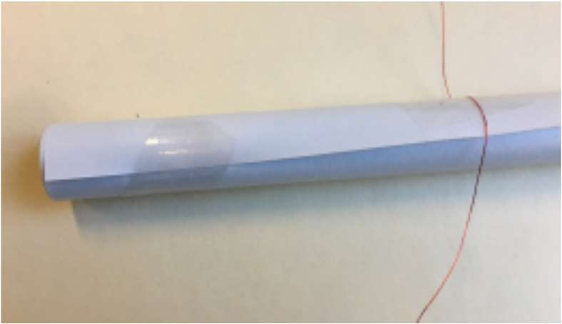
- Roll up a letter-size sheet of paper so that the axis of the cylinder that you get is parallel to the shorter side of the paper. Make approximately 5 turns. Secure the rolled-up paper with two pieces of Scotch tape, approximately 1.5 inch from the ends. Attach one end of the copper wire to the cylinder with Scotch tape, approximately in the middle of the cylinder (see Fig. 1).
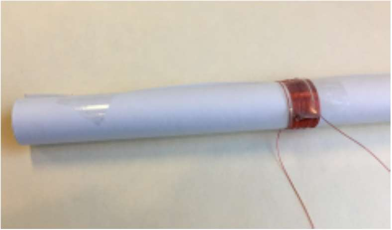
- Wind 30-40 turns of wire around the middle of the pipe to create a tight coil. It does not matter if the turns overlap. Leave about 6 inches of wire at each end free. Use a piece of Scotch tape to secure the coil (see Fig. 2).
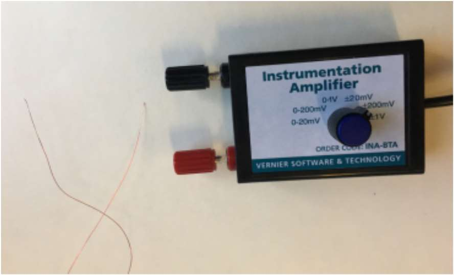
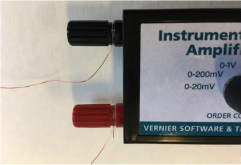
- Remove the insulation from the ends of the leads with the sand paper. Attach the leads to the terminals of the Instrumentation Amplifier and tighten the connection. Figure 3 shows the Instrumentation Amplifier before the connectors are tightened. Figure 4 shows the connectors with the copper wire attached to them.
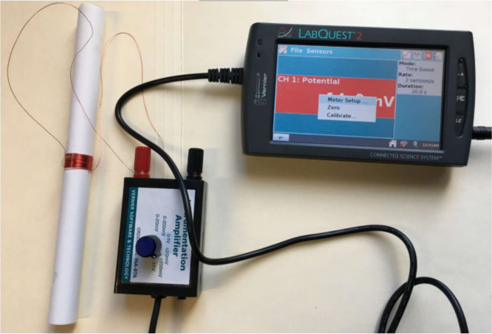
- Set the selector switch on the Instrumentation Amplifier to ± 200 mV. Connect the instrumentation amplifier to channel 1 of LabQuest2. Zero out the instrumentation amplifier. The signal should be 0mV or fluctuating around 0mV. If there are large fluctuation, take the copper wire off the contact and try to clean it more. Figure 5 shows the Instrumentation Amplifier connected to the coil right before zero-ing out the voltage.
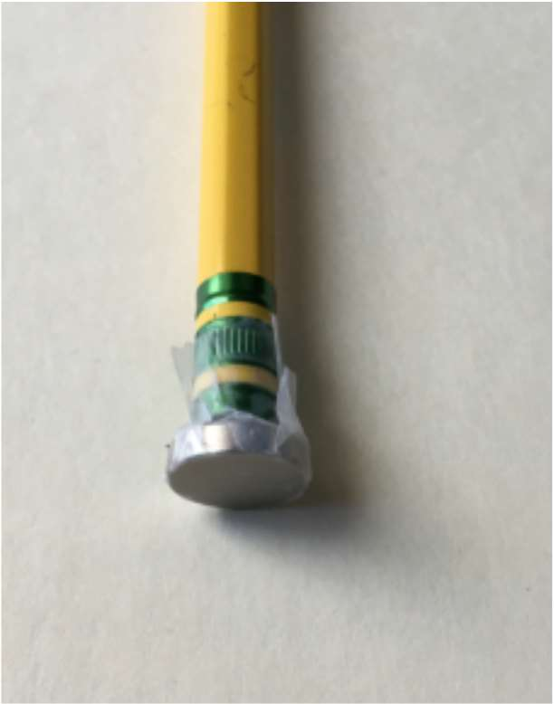
- Tape a magnet to the end of a pencil (see fig. 6). This will allow the magnet to pass through the pipe without changing orientation.
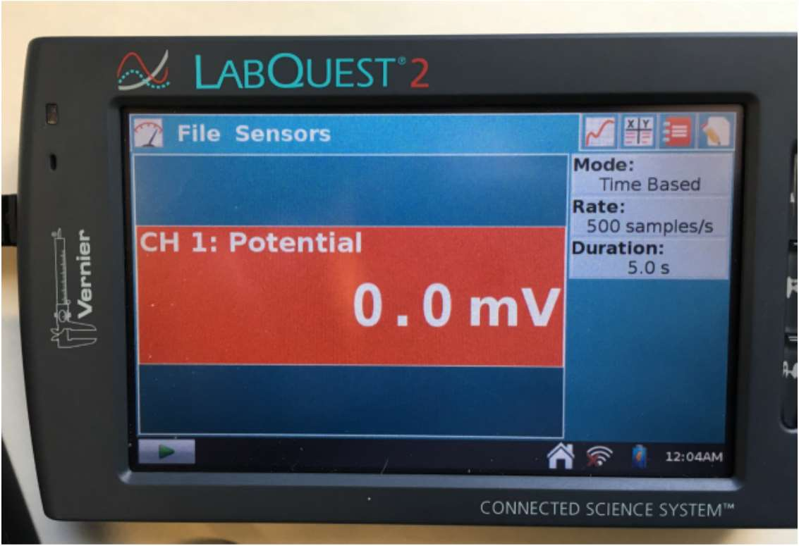
- Change the data-collection duration to 5 s and the data-collection rate to 500 sample/second or 1000 sample/second (Fig. 7).
- Mark one end of the cylinder as “top”. Make sure that you do not invert the cylinder between measurements. Tilt the cylinder at a shallow angle. Test to see that the magnet- pencil assembly moves smoothly through the coil.
- Start data collection, and then release the magnet. Store the run (Run 1).
- Increase the angle of the cylinder and repeat Step 5, but wait a bit longer to release the magnet. This will ensure that the graphs from the runs do not overlap when you view them all at once. Store the run (Run 2).
- Repeat Step 6 with an even steeper angle; store the run (Run 3).
- Perform a final run with the coil held vertically. Save the experiment file (Run 4).
- Invert the magnet on the tip of the pencil. Do one more run with the coil held vertically (run 5).
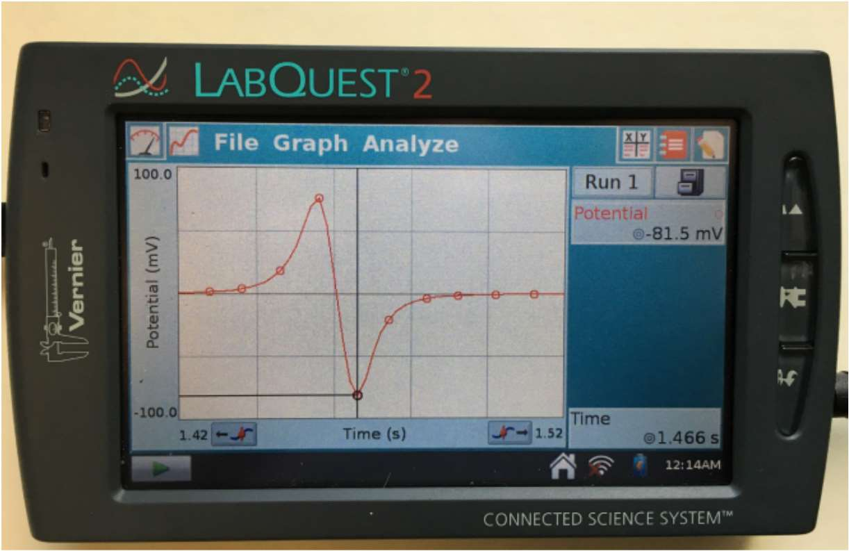
- For your first run, click and drag to select the region that shows the potential changing as the magnet approached, passed through, and then receded from the coil. Figure 8 shows a typical recording. (In your recording the negative and positive parts of the graph may be interchanged. That is not a problem.) To zoom in to the relevant portion of the recording click on “Graph” and then click on “Zoom in”.
- Click on the highest voltage point Figure 8 on the graph and record the corresponding potential, \(V_1\) , and time, \(t_1\) . Repeat that for the lowest voltage and record \(V_2\) and \(t_2\) .
- Calculate the time difference \(t = t_2 - t_1\) and the voltage difference \(\Delta V = V_2 - V_1\) . When calculating the voltage difference follow the positive/negative signs carefully. Calculate \(1/t\) and enter the value in Table 1. Note: LabQuest measures the time in seconds and it uses mV for the voltage. When calculating the time difference it is best to use units of ms.
- Estimate the error of \(V\), \(\sigma V\), and the error of \(t\), \(\sigma t\). To calculate the error of \(1/t\) use \(\sigma(\frac{1}{t}) = \sigma t /t^2\).
- Repeat this for your other runs.
| \(V_1\) mV | \(t_1\) ms | \(V_2\) mV | \(t_2\) ms | \(V\) mV | \(\delta V\) mV | \(t\) ms | \(\delta t\) ms | \( 1/t\) | \(\delta 1/t\) | |
|---|---|---|---|---|---|---|---|---|---|---|
| Run 1 | ||||||||||
| Run 2 | ||||||||||
| Run 3 | ||||||||||
| Run 4 | ||||||||||
| Run 5 |
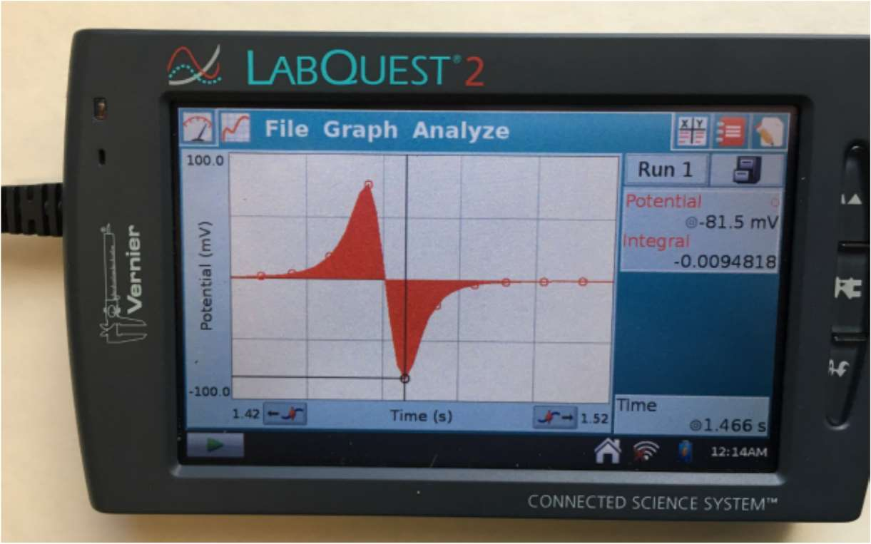
- For your first run, click and drag to select the region that shows the potential changing as the magnet approached, passed through, and then receded from the coil. Figure 8 shows a typical recording. (In your recording the negative and positive parts of the graph may be interchanged. That is not a problem.) To zoom in to the relevant portion of the recording click on “Graph” and Figure 9 then click on “Zoom in”.
- Click and drag to highlight the whole graph, starting from the left side, where the potential is close to zero and going to the right side, where the potential is zero again.
- Click on “Analyze” and then click on “Integrate” (see Fig. 9). Record the value of the integral in the “φ ” column of the Table below. (The integral is, by definition, the area under the curve. For the part of the graph where the potential is negative, the area is also negative. The proper unit of the integral is voltage times time, i.e. Vs. However, by inspecting Eq. (3) we see that on the right hand side we have magnetic flux, that has units of Weber, Wb. Therefore 1\(Vs\) = 1\(Wb\). LabQuest measures the time in seconds, but it uses mV for the voltage, therefore the number you read out is in units of milli \( Vs\) = milli \(Wb\) = \(10^{ -3}\) Wb.)
- Select the first portion of the curve when the magnet approached the coil but before the abrupt sign change in the potential. Choose Integral from the Analyze menu to determine the value of the area under this portion of the curve. Record the value of the integral in the \( \phi_1 \) column of the Table below.
- Copy over the values of \(1/t\) from Table 1.
- Repeat for Runs 2-4.
| \( \phi \) mWb | \( \phi_1 \) mWb | 1/t in per millisec | |
|---|---|---|---|
| Run 1 | |||
| Run 2 | |||
| Run 3 | |||
| Run 4 |
Answer these questions:
- The shorter is \(t\) in Table 1, the faster the magnet moves. The speed is proportional to \(\frac{1}{t} \). Based on Faraday’s law (Eq. 2) one expects a linear relationship between \(V\) and \(\frac{1}{t} \). Use the plotting tool to test this relationship. (Using the values in Table 1, enter \(\frac{1}{t} \) as “x” and \(V\) as “y”. Also enter the corresponding errors). Is the linear relationship satisfied within the experimental error?
- What is the total change of the flux \( \Phi \) between the time when the magnet started to move towards the coil (well before \(t_1\) ) and the time when the magnet completely left the coil (well after \(t_2\) )? Remember, when the magnet is far away from the coil the magnetic field at the coil is very close to zero.
- Based on your answer to the previous question, and using Eq. (3), what do you expect for the value of the “Total Integral”, \(\Phi\) , in Table 2? Does this value depend on the speed of the magnet?
- To compare your prediction to the experiment use the plotting tool, make a graph of the \(\Phi\) as a function of \(\frac{1}{t} \) (there is no need to enter the error of these quantities). Are the experimental results consistent with Faraday’s law? Link for Plotting Tool
- What do you think: where is the magnet relative to the coil at the moment when the voltage versus time graph crosses zero? At this moment, how large is the magnetic flux through the coil relative to the flux at other times? At this moment, is the flux changing with time?
- Based on your answer to the previous question, and using Eq. (3), do you expect a variation between the runs? Use the plotting tool to plot \(\Phi_1\) as a function of \(1/t\) (there is no need to enter the error of these quantities). How accurately does your expectation correspond to the experimental results?