The purpose of this lab is to study Newton’s second law using an Atwood’s machine, and to apply the law to determine the acceleration due to gravity experimentally. This will be done by exploring the relationship between the acceleration, tension, and the masses in the apparatus. ^{Hoveroverthese}

Equipment

• LabQuest 2
• Vernier Photogate
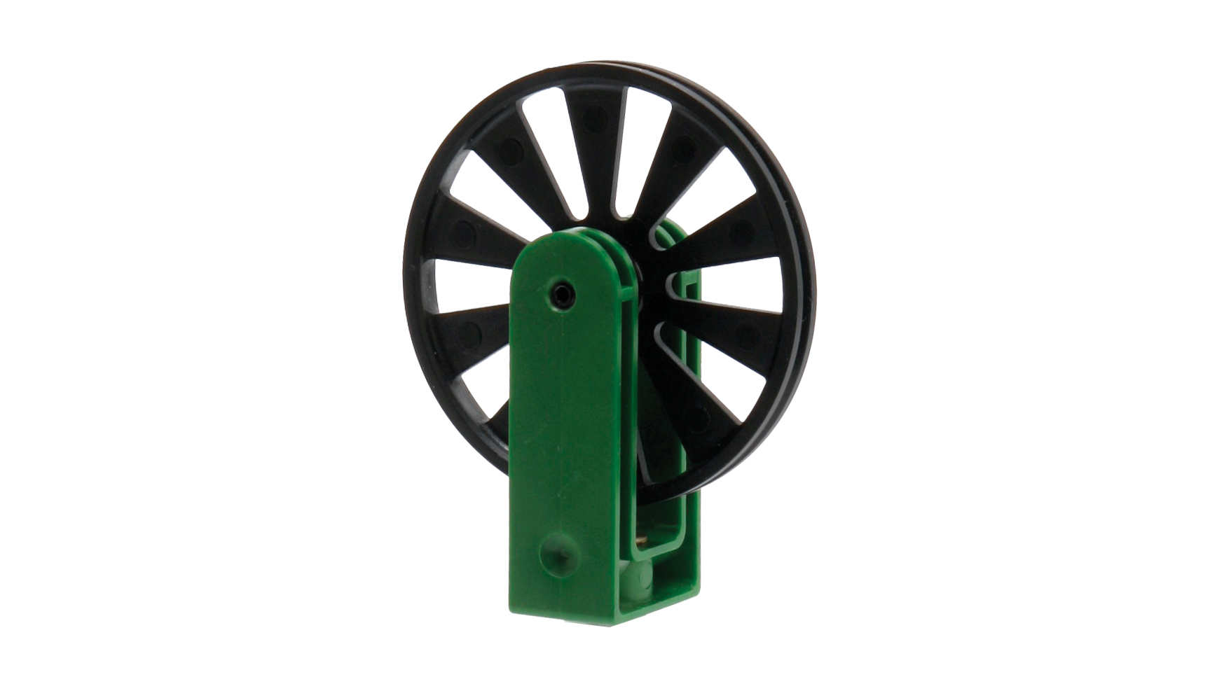
• Ultra pulley (negligible mass)
• Mass set
• Lightweight string
• Stand and clamp

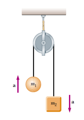
An Atwood’s Machine consists of two objects of different masses hanging vertically over a frictionless pulley of negligible mass. When the system is released, the heavier mass accelerates downward while the lighter mass accelerates upward at the same rate. The masses are connected by a light string so we assume the tension is the same in each part of the string. The acceleration, which is the same for both masses, depends on the masses of each object as well as the gravitational acceleration constant.

To solve it, let’s separate the system into two smaller systems, where each system consists of one mass, and apply Newton’s second law for each system. Since the movement of each object is just in the vertical direction, we only need to calculate the net force in the “y” direction for each object. To determine a sign convention (which direction is positive and which is negative) for this problem is important, since each object is part of a separate small system, we can assign a different sign convention for each system. The recommendation is always to pick the positive direction as the direction of the acceleration in the system. In this way, according to previous figure, object 1 of mass m 1 has an upward acceleration, then the reference is positive in the upward direction. And for object 2 of mass m 2 , the reference is positive in the downward direction, because of the downward acceleration.

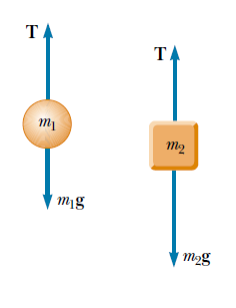
Applying Newton’s Second Law based the free-body diagrams to the left, the equation for systems 1 and 2 are: $$ Object m_1 : \Sigma F = T − m_1 g = m_1a_y $$ $$ Object m_2 : \Sigma F = m_2 g − T = m_2 a_y $$ Note that the tension and acceleration of the two systems are exactly the same, because they are connected through the same lightweight string and the pulley is frictionless and has a neglected mass. Working with equations (1) and (2), the expressions for the tension and the acceleration are $$ T= \frac{2m_1m_2}{m_1 + m_2} g $$ $$ a_y = \frac{m_1 - m_2}{m_1 + m_2} g = \frac{m_{diff}}{m_{sum}} g $$ It is your job to work with equations (1) and (2) and check the validity of expressions (3) and (4).

1. Connect the photogate to the digital channel port of the LabQuest2 and check that it has the right setup for this experiment. On the right of the meter screen (Tab A) you will find a data-collection details row; verify that the “mode” says “photogate timing”, click in the mode option, and in “photogate mode” select “motion” and choose the “pulley ” – “outside edge” option. Choose “end data collection” and select 25 events.
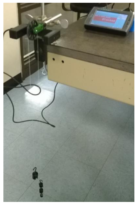
2. The figure shows the setup of the apparatus. Note: The masses must be able to move at least 50 cm before hitting the ground.
3. Connect masses on each side of the string while holding the wheel stationary. Steady the masses so they are not swinging. The combination of masses that you will use in each trial is shown in the next table. Each combination of masses represents a trial and you will repeat each trial twice.

   Trial	1	2	3	4	5
   \(m_1\) (grams)	40	70	10	20	20
   \(m_2\) (grams)	50	100	20	50	100

4. Select the “graph screen” (Tab B from previous figure) and click “collect” to start data collection.5. Release the system and stop it before the falling mass hits the ground (the other mass will hit the pulley if you do not stop the system).
5. Take the graph of velocity vs. time and fit a straight line to your data. To do this, select the data on your graph and go to “analyze” and then “curve fit.” Select “linear“ in the fit equation option, and then click OK. Record the values of the slope “m”. What does this value represent in this graph? (use variables from equations 1-4 to answer this question).
6. Repeat steps one more time with the same combination of masses.
7. From the two values of slope, find the average value of the slope.
8. Change the masses on each side of the string according to the table and repeat steps from 3 to 9.

Determine experimentally the gravitational constant

Use the web based plotting tool to plot the average acceleration for each trial as “y”, and the values of \( \frac{m_{diff}}{m_{sum}}\) as “x” or in other words, plot acceleration vs. \( \frac{m_{diff}}{m_{sum}}\). Don’t forget to enter the uncertainty in the acceleration values you calculated earlier and chose to include this on your plot. You can consider the uncertainty to be the difference between your two measurements for each trial. The calculated slope from the fit represents the gravitational constant, and the program also gives a value for the uncertainty in the slope. Is your value for \(g\) consistent with the accepted value of \(g = 9.81 m/s^2\) ?¹

Answer the following questions:

1. What would the acceleration a y of the system be if the masses of the objects 1 and 2 are equal? (\( m_1 = m_2\) ). What would the tension T of the string be?
2. Assume that you will do the experiment one more time, but, instead of simply releasing the system, you give a short impulse by pulling the heavier mass downward and then let go of it. In the LabQuest2 you analyze the region of the velocity vs. time graph right after the impulse duration.
   1. How would the value of acceleration change compared to your previous measurements for the time interval after the impulse?
   2. What happens if you instead give a short impulse in the other direction by pulling the lighter mass downward and then let go of it?

Guide to Uncertainty Propagation & Error Analysis (Quick Reference)

PHY121/122 Plotting Tool

PHY131/132 Plotting Tool