In this lab exercise you will gain a working knowledge of how to use an oscilloscope by measuring the amplitude of a square wave and the frequency of a sine wave.

Note that the goal of this experiment (from a learning perspective) is largely to give you an understanding of this (somewhat complicated) instrument, so that we can use it in future experiments without requiring further explanation. As such, there are questions in the procedure that you don't need to formally answer in your report, but should make sure you understand (for your own sake).^{Hoveroverthese!}

• 1 Oscilloscope (2 Banana/BNC Adaptor LEAVE CONNECTED)
• 2 Function Generator (2 Banana/BNC Adaptor, 1 each, LEAVE CONNECTED)
• 4 Banana cables, 2 Alligator Clips
• Record data in this Google Sheets data table

A description of how the oscilloscope works can be found here: Oscilloscope Description ¹

A description of how the function generators work can be found here: Function Generator Description

In short, the oscilloscope is going to measure the voltage difference between the red and black wires plugged into it and plots this voltage (y-axis) as a function of time (x-axis). This is what appears on the oscilloscope screen.

In more detail: the oscilloscope starts by outputting a dot at the left-hand side of the screen, and moves up and down with the voltage input as it moves to the right. Then, it jumps back to the left, and draws it again. If it moves fast enough (which it will, given how we'll be using it), this will look like a curve as it moves across the screen. Each of these "screen crossings" is called a horizontal sweeep.

In older, so-called "analog" oscilloscopes, the physical mechanism by which the dot is made on the screen is similar to a CRT TV in that an electron beam (emitted from an electron gun at the back of the device towards the front) hits a phosphor-coated glass screen. The location of the dot is determined by a pair of vertical and horizontal deflection plates which use electric fields to deflect the electrons in the vertical and horizontal directions, respectively, to have the electron eventually collide with the correct point on the screen.

In the oscilloscope we will use, the voltage difference between red and black wires ("signal" and "signal common") is digitized into a 8 bit number at one billion samples per second (1 GSa/s). The device can store 56 million measurements at a time (56Mpts) which means that it can retain only a small fraction of the values it acquires in one second. So, this device is best suited to look at signals which vary over short times: milli, micro or nano seconds.

The process to decide which digitized values to display is designed to best show repeated waveforms; accordingly, our instrument has to ensure that it starts at the same point on the wave each time. The way it does this is using what we call a trigger - it only starts a sweep when the voltage crosses some fixed value. We control the trigger to investigate the aspect of the signal which is of interest to us (the "leading edge" or "falling edge" or "runt signal", etc).

The oscilloscope can actually analyze two signals at the same time, input via two different channels. Later in this course, we'll use this to compare an "input signal" and a "system response" (of various sorts). In this lab, though, we'll just be comparing two separate input signals, both by putting them on the screen at the same time and using "XY mode" to make a plot of one voltage versus the other (without time information).

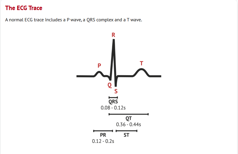
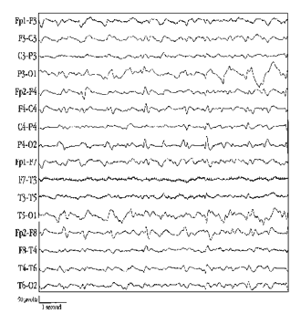
An oscilloscope may seem to be an instrument which only interests physics-types and electrical engineers. However, an oscilloscope is the basis of many devices which apply a sensor and observe its time dependent output. Two examples are an ECG and EEG, seen below.

Basic Oscilloscope Setup

Begin by unplugging any red or black cables from the front of all devices, before you turn anything on. Please leave the Banana to BNC adapters on the function generator and oscilloscope.

Let's first get the oscilloscope to a good "default" position for getting some basics down:

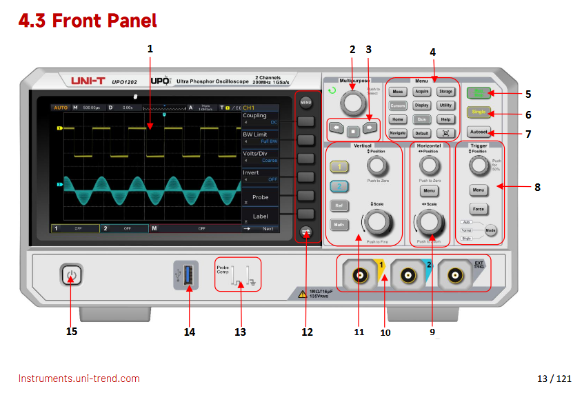
• Press in the power button (lower left of the unit, below the screen).
• Watch the light show as the oscilloscope initializes.
• Ready to go! If you are confused about the operation of the device, one can always return to the initialize function by pressing the button "Autoset", in the upper right region of the oscilloscope.

So, at this point you should just see both yellow (Channel 1) and blue (Channel 2) traces on the screen. They will be "noisy" because the adapters are acting like antennae for small signals in the environment.

Put an alligator clip in one end of a red banana cable. Insert the banana end into the red connector on Cha 1. Use the alligator clip to connect to the Ground Clip of the Test Output (rightmost connection on Box 13 in the above photo) . The trace of Cha 1 will now be a flat, yellow line at Zero Volts. Do the same for Cha 2 (and get a flat blue line).

Vertical Position and Channel Control

Press the yellow lit button for Channel "1". See that a menu appears which is about how Cha 1 is connected to the device. The Cha 1 vertical scale indicator will be lit in the lower left of the screen.

Press the yellow button for Channel "1", again. This turns off the display of Channel 1.

Press the yellow button for Channel "1", yet again! This turns on the display of Channel 1.

Do the above steps for Channel "2".

Now, use the Vertical Position knob to put the yellow trace above the blue trace, then put the blue above the yellow.

This might seem strange: if we can freely move the traces up and down, how does that result in a "measurement"? We can set it to anything we want!

This is partially true, but usually for this kind of signal, we only care about the variations in voltage, or we know that they average out to zero (like a sine wave). The variations are directly measureable, so that works fine.

Moreover: if we want to measure the voltage on an absolute scale, we can measure zero by flicking the left-hand switch to GND briefly, so we could measure absolutely if we wanted to - perhaps even set GND to the middle of the screen. (In this class, though, we won't ever need to to this - we'll only ever be interested in the variations, for which we won't need to know what "zero" actually is.)

The ability to move stuff around is primarily so you can put it into a nice part of the screen to look at. (For one signal, this might seem esoteric, but when you have two signals on the screen at the same time, it can be useful.)

Setting Up a Square Wave

Move the alligator clips from the Ground connection to the compensated proble connection (Probe Comp). Add black wires from the black ("GND" or "signal common") connector on Cha 1 and Cha 2 to the Ground Clip. Red going to the signal of interest and black going to ground (signal common) is the usual way one connects circuits.

Ensure that the alligator clips from "Probe Comp" do not touch the clips in Ground. This "shorts out" the circuit and just makes all voltages zero. ¹²

Using either Cha 1 or Cha 2, use the Vertical Scale knob to find the signal on that channel. This should be a "square wave". Likely, you will need to set the Vertical Scale to 1,2 or 5 Volts, which means that every vertical box represents 1,2 or 5 Volts (often called "volts per division"). Now, do the same for the other channel.

Likely, you will just see two horizontal lines on each of Cha 1 and 2. This is because the signals are not "triggered". For now, use the "Autoset" button to have the oscilloscope make decisions for us. You should now have two nice square waves.

Horizontal Position and Scale

Try the Horizontal Position knob (Sector 9). You will see the traces move left and right. Note that the small arrow labelled "T" above the traces moves: this is the point (in time) where the trigger occurs. Times to the left are "before the trigger" and times to the right are "after the trigger".

The Horizontal Scale knob sets the length of time that one horizontal box describes. (Note: one box, not one tick mark.) This is often caled the TIME/DIV (time per division).A "division" is one box.

Right now, you should observe that one period of the wave is two boxes. Look to the upper left of the screen: "M" says 500 \(\mu\)S, so one box is one 500 \(\mu\)S. Therefore, the period of the wave is one millisecond.

Since \(f=1/T\), we can calculate the frequency. Since 1/(1ms)=1kHz, the frequency of our square wave is therefore 1kHz. You will see that the use of Autoset turned on a frequency measurement, which displays 1 kHz in the upper right of the screen. The frequency of this square wave is 1kHz. So it matches what we expect!

Turn the Horizontal Scale knob by a click or two. Check real quick: does the result still make sense on this new setting? That is, find the period of the wave (new Time/Div and new number of divisions) and calculate the frequency. Is it still the expected 1kHz? This isn't to hand in, just to get settled with the idea of the measurement.

Now, return to the vertical setting: VOLTS/DIV. This is the same idea on a different axis. As our first measurement, we'll check whether the amplitude of the square wave is what we expect.

Part I: Square Wave Amplitude

Turn off Channel 2 and use Channel 1 for this part.

Adjust the square wave with the POS settings and the VOLTS/DIV setting until your screen is almost entirely filled with a few periods of the square wave. Record the VOLTS/DIV and TIME/DIV on your data sheet for later reference.

On the paper provided, sketch a copy of what you see on the oscilloscope screen.³

Now: count the number of boxes vertically from the bottom of the grid on the screen to the bottom of the square wave, and record this on your data sheet as your "low reading." (Count the big boxes, not the little tick marks.) Round to the nearest half-tick-mark. Estimate your uncertainty in this reading based on how precise you think your measurement is (generally at least 0.5 tick marks).

Repeat this measurement, except this time counting from the bottom of the grid to the top of the square wave, and record this as your high reading.

Using your VOLTS/DIV, convert these to the physical upper and lower voltages for the square wave. The difference between these will be the "peak-to-peak" amplitude of the square wave.¹

We will compare this amplitude to the expected amplitude of 3 Volts. Record this expected amplitude on your data sheet.

Part II: Sine Wave Frequency

Refer to the Reference Guide for Function Generators for this part. You will need to identify what sort of function generator you have in order to know how to use it correctly. Instructions here are for Juntek or Koolertron (essentially identical) models.

Remove the alligator clips and detach all 4 wires from the Probe Comp output of the oscilloscope.

Turn on your function generator and wire its Channel 1 (yellow) and to CH 1 of the oscilloscope (red to red and black to black).⁴

Set your function generator to output a sine wave at a frequency of 3.1 - 3.4 kHz (3100 - 3400 Hz) . You choose .⁵

Use the Trigger menu (Sector 8) to select Channel 1 for your trigger. Push the Trigger Position knob, the oscilloscope will "trigger" its display at a "zero crossing" of the sine wave (with positive slope).

Adjust this sine wave (with Vertical Position and Scale) and until it takes up most of the screen vertically and you have ~3-8 periods of the wave on screen. Record the VOLTS/DIV and TIME/DIV on your data sheet for later reference.

Sketch the sine wave you see on the paper provided as you did for the first measurement.⁶

We'll now measure the time it takes to complete the periods you have on screen. Choose some point on the first oscillation you see to measure from (say, the top of the peak). Count the number of waves between that point and the corresponding point on the last wave on your screen. Record this as the number of waves. (Be careful not to get an off-by-one error!)

Now, record the number of boxes from the left edge of the grid on the screen to the point where you started counting waves as your start reading. Similarly, record the number of boxes from the left edge of the grid to the point where you stopped counting waves as your end reading. Note unlike before, we're counting horizontal boxes this time, not vertical boxes.

Understanding Triggering

Begin set up with the sine wave (per the previous part). Now, turn the horizontal position knob to the right by a couple of boxes (divisions) and then left. Observe that the "trigger point" (indicated by the small arrow with "T" on it) moves.

Next, adjust the Trigger Position knob up and down a little bit. What happens to the starting point on the wave? What happens when you turn the trigger level up too high (or down to low), above the top (or below the bottom) of the wave?

Now, set the trigger position back to a "reasonable" level. Select the Trigger Menu and try three values of "Slope" (Rise, Fall, Rise & Fall). What happens to the starting point now?

Finally, use the "Wave" menu on the function gnerator to try a triangle or square wave (and vary the TRIG Position knob, etc.)?

Analyzing Two Signals

Plug Cha 1 of your function generator into Cha 1 of the oscilloscope and Cha 2 into CH2.

Have both your function generators set to similar frequency sine waves (but not exactly the same). Now, look at your screen: you should see two sine waves. (If you don't, ensure that both function generator outputs are On and that both Cha 1&2 of the oscilloscope are On). One of them should be moving.

Look at both: which one is "stable" and which one is "moving"? What if you change the Trigger Menu (Sector 8) SOURCE from CH1 to CH2?

Finally, vary each VOLTS/DIV knob. What does each knob do to each signal? What about TIME/DIV and horizontal position? (Which knobs alter both curves, and which knobs alter them separately?)

Lissajous Figures

Now for one last feature of the oscilloscope (which we won't be using again in this class, but is still pretty neat): use Horizontal menu (Sector 9) to set the Time Base to X-Y.

This plots the two voltages against each other (time is no longer an axis) - the dot now has its (x,y) position determined by the (CH1,CH2) voltages.

Try these:

• Set the frequencies of Cha 1 and Cha 2 of the function generator to the same value;
• Set frequencies of Cha 1 and Cha 2 of the function generator to the nearly the same value: 0.1 Hz different;
• Set the frequencies of Cha 1 and Cha 2 of the function generator to the same value and vary the Phase difference (available on Cha 2 of the function generator). Interesting points are phase differences 90\(^o\), 180\(^o\), 270\(^o\) ;
• Set the frequencies of Cha 1 and Cha 2 of the function generator to the an integer ratio, such as 3:2 or 4:3. Add 0.01Hz to one of the channels. What do you observe?

Understanding this is mostly just the math of parametric curves, but it's still pretty to see.

Take note of the shapes you see (draw on oscilloscope sketch paper, take pictures, whichever), along with what frequencies made that shape.

Understanding The Rest (Optional; No Procedure)

Finally, please turn off all the electronic equipment before you leave the lab. Do this for all labs in this course.

Oscilloscope Sketches

In this lab, you will make two oscilloscope sketches. Each of them should have the following:

• A title for the plot.
• Labelled axes, with units: "Voltage (V)" for the y-axis and "Time (s)" for the x-axis (with the units changed if you use mV, ms, or μs instead of V and/or s - choose appropriately for your Volts/Div and Time/Div settings).
• Numbered axes: choose an (arbitrary) origin for your plot, and put numbers on your axes, where the numbers correspond to physical quantities. That means you should use your Volts/Div setting to determine the y values and the Time/Div setting to determine the x values.
• A sketch of the curve that is visible on your screen (of course), drawn to the best of your ability.

You should ignore the little 0/10/90/100 numbers on the left side of the screen: none of those are relevant.

On the Data Sheet

You should show the following calculations, with error propagation for each:

• Part I:
  • Convert your vertical "box" measurements into physical voltages.
  • Take the difference of your physical voltages to measure the "peak-to-peak" amplitude of the square wave.
• Part II:
  • Convert your horizontal "box" measurements into physical times.
  • Take the difference of these times to calculate the total time for multiple waves.
  • Divide by the number of waves that occur in that time to get the period.
  • Take one over the period to get the frequency.

Based on the data you extract in this part, answer the questions in the data table about the compatibility of your results with expectation.

Your TA will ask you to discuss some of the following points (they will tell you which ones):

• Functions of the Oscilloscope: Describe, in your own words, what the following components of the oscilloscope do and how to use them:
  • Plot visual controls (POS, VOLTS/DIV & TIME/DIV)
  • Triggering (basic idea of what it does, TRIG LEVEL, SOURCE)
  • Two inputs (CH1 vs. CH2 controls [what they share, what differs], VERT MODE, XY)
• Analyzing Lissajous Figures: Answer these questions about the last part assuming the function generators are always outputting sine waves.
  • Same Frequency, special cases: What do you expect to see if the two function generators are at exactly the same frequency and in-phase? What if they are out of phase (by 180 degrees)? What if they are 90 degrees out of phase?
  • Same Frequency, general case: In general, what do you expect to see if the two function generators are at exactly the same frequency with arbitrary phase?
  • Perfect n:m ratio: Suppose the two frequencies were exactly in an integer ratio (2:1, so one is twice the other; 3:2, so one is 3/2 of the other; etc.). What do you expect to see (as a static image) in this case? (Again, you may consider phase shift as well.)
  • Frequency Difference: Now suppose they are at almost the same frequency, but slightly different. What do you expect to see here? (Hint: note that \(\sin(\omega_2 t)=\sin(\omega_1 t+(\omega_2-\omega_1)t)\); hence, if your two frequencies are similar, the second input looks kind of like the first with a slowly-varying phase shift.) Does this align with what you actually saw?
• Triggering for Other Purposes: One important use of an oscilloscope is as a sort of particle detector for phenomena like radioactive decay. A radioactive decay response generally looks flat, except that at random times there's a "bump" (of some more-or-less-fixed shape) from a particle detection from time to time.
  • Triggering Usefulness: Unlike our inputs in this experiment, which are periodic, radioactive decay occurs at random times. If we didn't use triggering in any way, we would see a mess on our oscilloscope screen. How can triggering be used to "organize" the radioactive decays into a single more-or-less stable waveform?
  • Limitations: In an analog oscilloscpe there is a key limitation, based on the fact that the trigger starts the scan. What is this limitation, and what does it prevent us from doing? Hint: this modern, digital oscilloscope is continuously digitizing, including "before" the trigger event. ⁵

Guide to Uncertainty Propagation & Error Analysis (Quick Reference)

Notes on the Oscilloscope

Notes on the Function Generators

Spare Oscilloscope Sketch Paper