SBU Intro Physics Labs, PHY 133 Standing Waves Lab

Department of Physics and Astronomy, Stony Brook University

Stony Brook University | Introlabs Main Page | PHY 133 Webpage

PHY 133 Laboratory
Standing Waves

TABLE OF CONTENTS

Introduction

Equipment

Background

Procedure

Analysis

Discussion Topics

References and Tools

Introduction

In this lab, we will study standing waves on both stretchy and rigid string.^Hover^over^these!

Equipment

1 function generator (Koolertron or Instek) ¹
2 Banana cables, red & black
1 Pasco Mechanical Wave Driver (SF-9324 or WA-9855)
2 Strings: 1 Stretchy (White), 1 Non-Stretchy (garish green)
1 Pulley + 1 string support stand (used with SF-9324 only)
Various Masses (can combine to 50-250 grams in steps of 50)
1 Meter Stick
Access to a Scale
Record data in this Google Sheets data table

Background

Basics of Standing Waves

Suppose you have a long horizontal string.¹ Suppose the string is under tension $F_T$ and has a linear mass density (mass per unit length) of $\mu$ (both of which are independent of your position along the string).

If the string is "free" (or you look far away from the endpoints), then you will find waves that "propagate" along the string with some speed $v$.¹ This speed can be calculated in terms of the parameters of the string:²

$$v=\sqrt{\frac{F_T}{\mu}}$$

We will not be looking at this case, but the velocity $v$ is a key parameter of the string regardless. We will instead be looking at standing waves, which is what happens when we hold the string still at both ends.²

A special class of solutions in this case are the harmonics. These are sine functions that oscillate with a frequency $f$ and a wavelength $\lambda$. This means that your vertical³ oscillations make the string have a vertical position $y(x,t)$ of:

$$y(x,t)=\sin\left(\frac{2\pi x}{\lambda}\right)\left[A\sin(2\pi ft)+B\cos(2\pi ft)\right]$$

The velocity is then related to the frequency and the wavelength according to the simple formula:

$$v=f\lambda\label{veqfl}$$

The zeroes of the above function, $x=\frac{m}{2}\lambda$ (for $m$ any integer), are known as the nodes of the wave. The "flat" points (maxima/minima), $x=\frac{m+\frac{1}{2}}{2}\lambda$, are known as the antinodes.

Note that the endpoints of the string, $x=0$ and $x=L$, are both always nodes (since we hold those points still), meaning that there is some integer $n$ for which $L=\frac{n}{2}\lambda$. (We use $n$ to refer to the specific integer $m$ that gives the zero corresponding to $x=L$.)

In general, we know that $\frac{L}{\lambda}$ is the "number of wavelengths" that fit into our string length. This means that exactly $n/2$ waves fit into our string, which means that there are $n$ "half-waves," or equivalently, $n$ antinodes.

Hence, if we fix $L$, we can state what wavelengths are possible, because they always have to correspond to some integer number $n$ of antinodes, and these wavelengths take the form:

$$\lambda_n=\frac{2L}{n}$$

Combining this with formula \eqref{veqfl}, we can find a formula for the $n$th fundamental frequency:

$$f_n=\frac{v}{2L}n$$

You may (quite fairly) wonder about the general behavior: what about solutions that are not these special harmonics? It turns out that these can always be written as a sum (or, more accurately, linear combination, or superposition) of these harmonics: a general vibration is a combination of these oscillations.

Thus, studying these special cases allows us to understand general vibrations, too.⁴

Experimental Setup

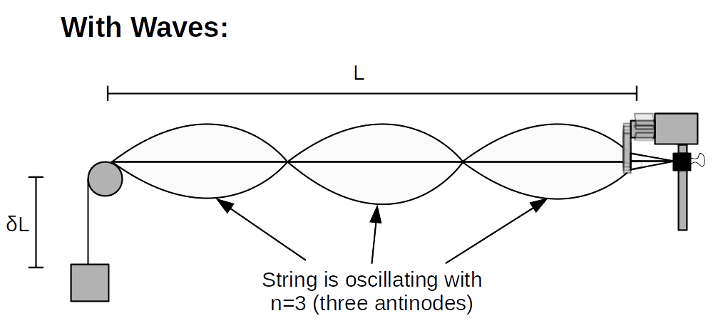
Schematically, the experimental apparatus that we will use to do this looks as follows:

Click to expand images of the apparatus

The Function generator with default settings — The function generator in default settings and the wave driver with stretchy string

Pasco wave drive with stretchy string, connected to function generator — The function generator in default settings and the wave driver with stretchy string

The pulley with hanging mass — The pulley with a hanging mass and stretchy string. The wave driver with some of the stretchy string, showing one antinode

Wave driver and some of the string, showing one antinode — The pulley with a hanging mass and stretchy string. The wave driver with some of the stretchy string, showing one antinode

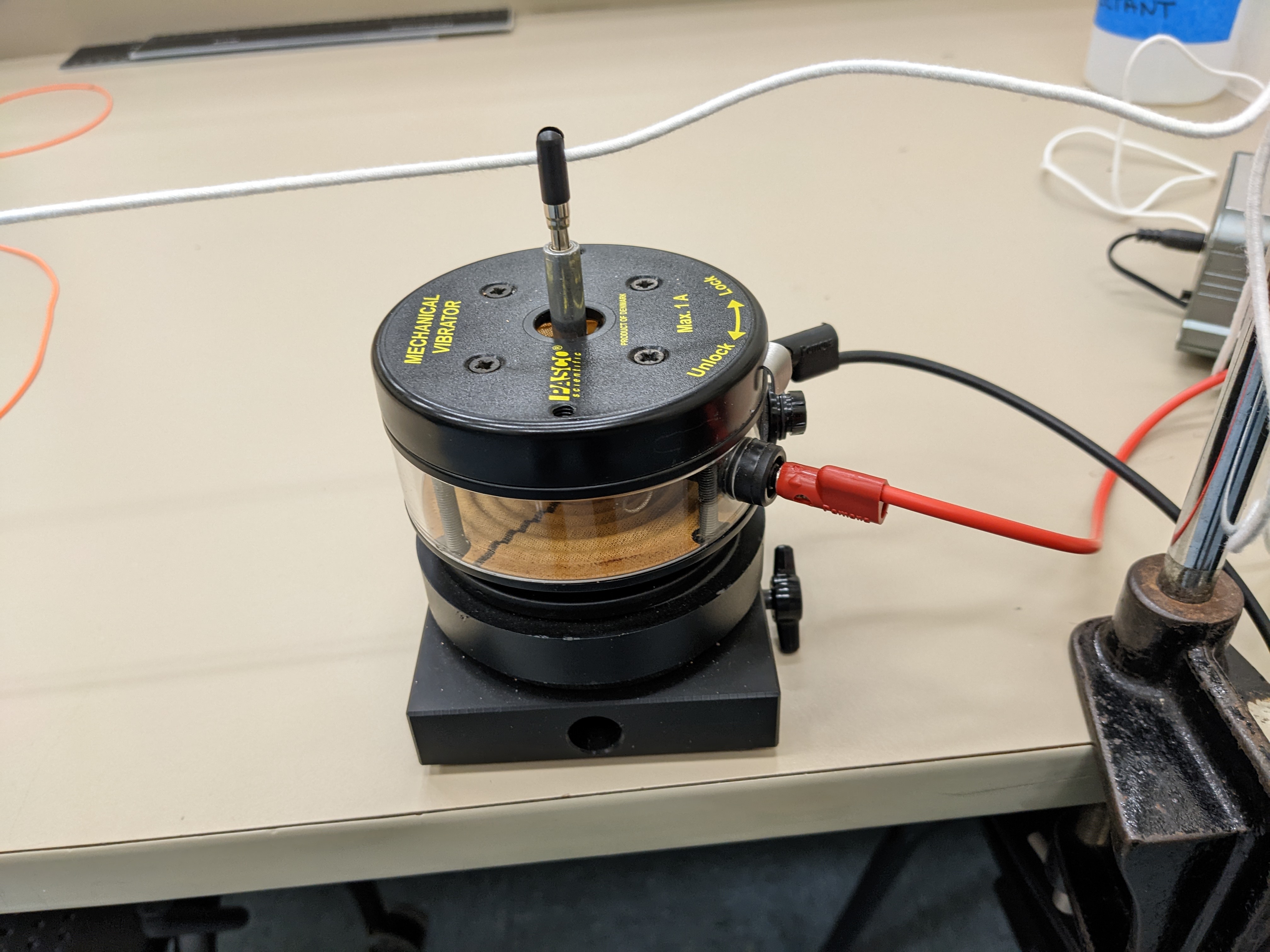
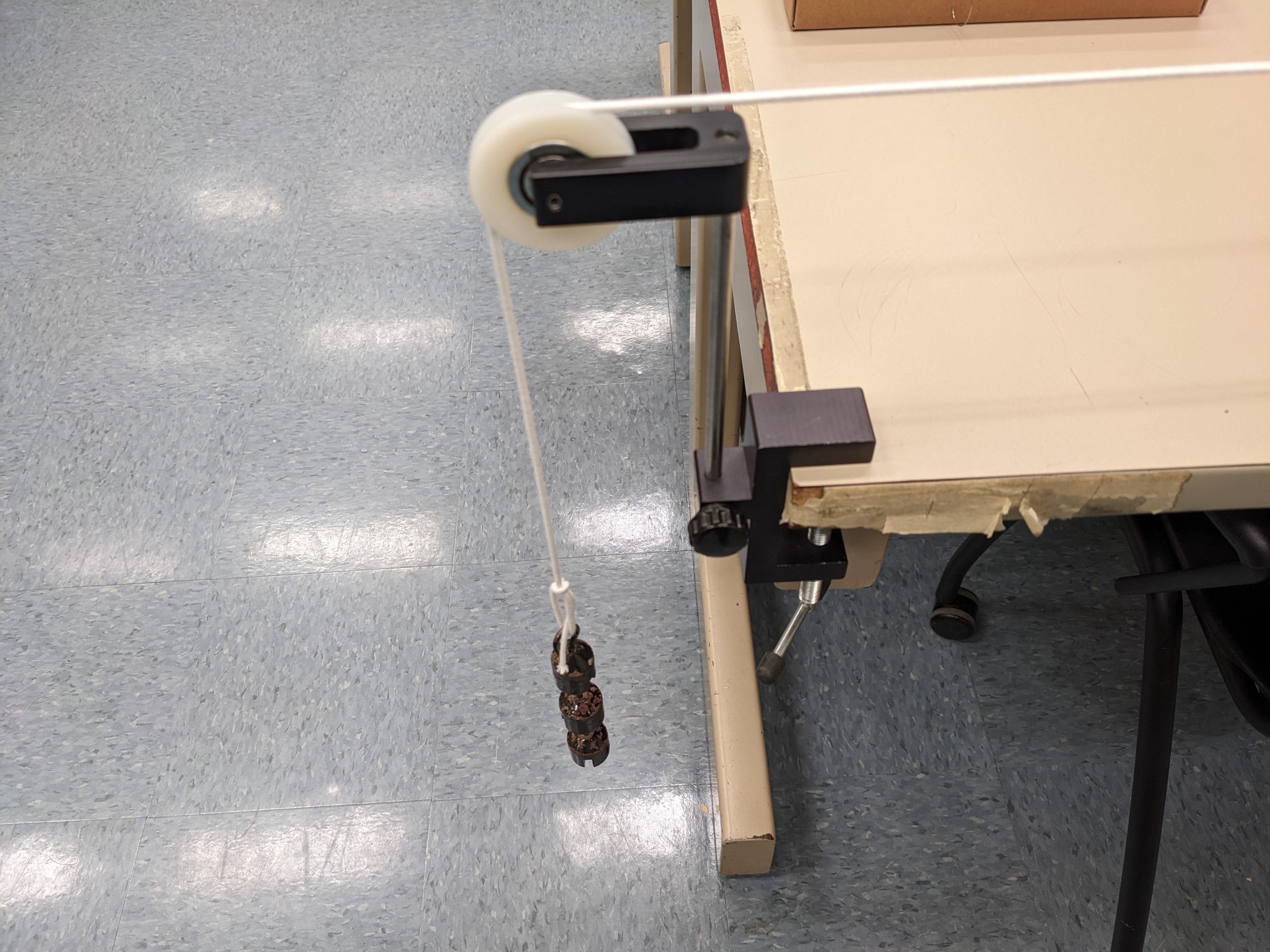
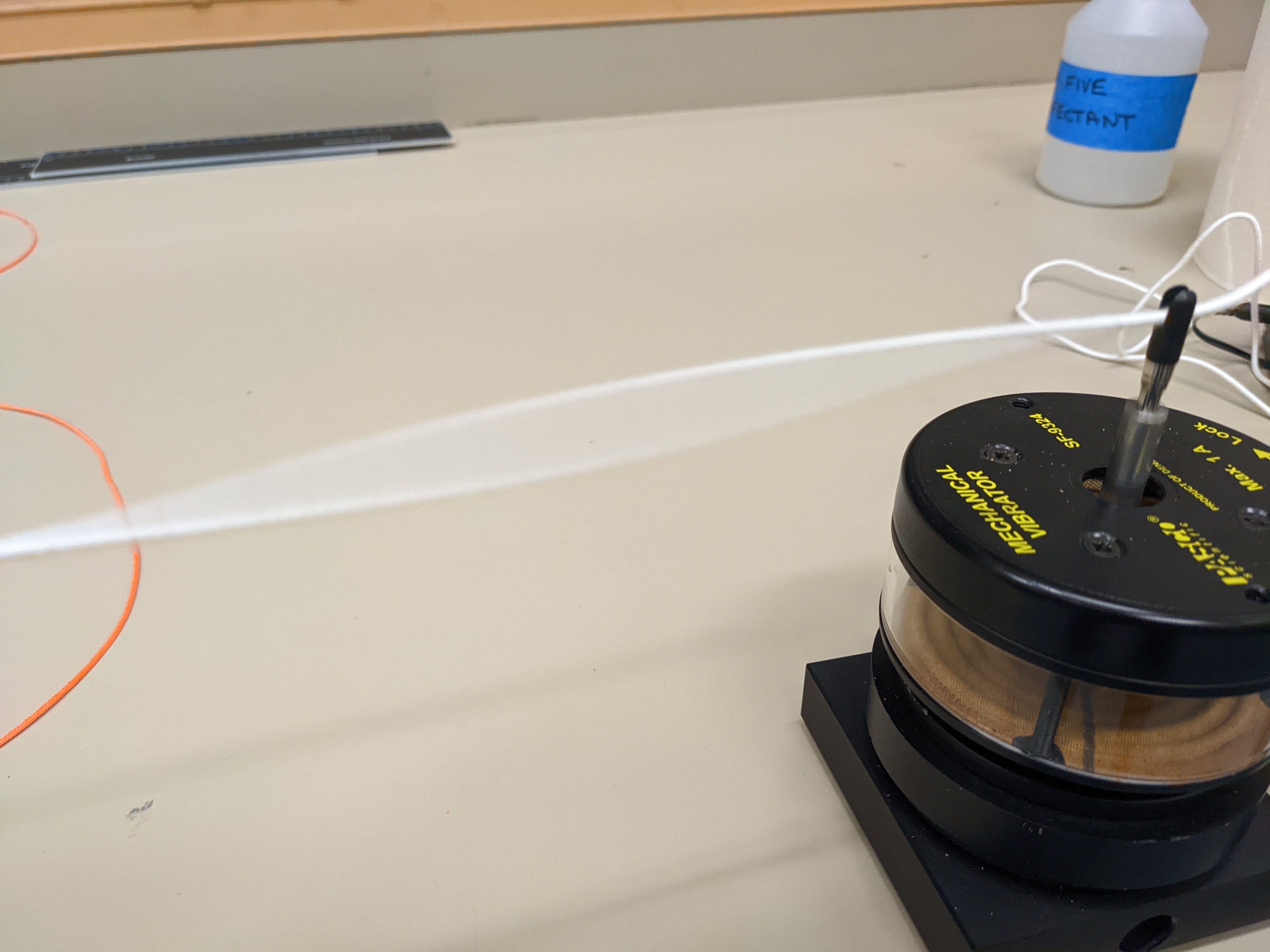
The hanging mass $M$ will determine the tension $F_T$ in the string. Note that in the last part (with the fixed-length string), we will vary this mass, where we should observe the relation:

$$f_n^2=\left(\frac{n}{2L}\right)^2\frac{g}{\mu}M\label{fnsq}$$

Note that the length of the string, $L'$, is just for the measurement of mass density. The oscillations themselves don't care about the string $\delta L$ beyond the end of the pulley; we treat the pulley as a fixed point!

Click here for some discussion about the role of the wave driver in this experiment

A significant technical subtlety (which we will not devote too much time to) is the fact that the waves here are not "free."

In other words, we don't have the ideal scenario, where the wave is somehow set to a single harmonic and allowed to oscillate freely. Instead, we are driving the wave by pushing it with a "wave driver".

The driver will oscillate with a frequency dependent on the power input. If this matches one of the harmonics of the string, then the whole string will oscillate with that harmonic, as we hope.

If the driver is near a harmonic, the wave will oscillate with something that looks like that harmonic, but the amplitude will be smaller. (The phenomenon that the amplitude is maximal when the driving frequency matches the natural frequency is known as resonance.)

If the driver is at some random frequency, the behavior is complicated, and so we will not be studying such a case in any detail.

A "proper" account of the driver would be to consider the motor as a fixed point of known oscillation frequency. I.e., rather than holding the endpoint fixed, we say that we know how the string behaves at the motor (and the other endpoint), and calculate what happens in between.

If the driver oscillates with a frequency that resonates with the rest of the string, then the answer is simple: you get the standing wave. (Basically, all other oscillations have friction in the string to contend with, and so slowly damp to zero; but when you consider the "right" frequency, the driver is pumping in energy to counteract friction, so that oscillation "stays steady.")

Otherwise, you have to solve the equations for waves on a string with known endpoints (not time-independent). Generally speaking, this is doable, but is too hard for us to tackle in this class.

Procedure

Part I: Predicting Stretchy-String Wave Velocity

Begin by taking your (white) stretchy string. Weigh it (the full length) on a scale to determine the mass, $m$. Measure and record the total length $L_{total}$

Identify if one end has a loop. If one end does, grab the other end; if neither end does, grab either end. Push the string into the black plastic piece on top of your Mechanical Driver. Then, clamp the extra string to the string support post with a "library clip". ²

If your string does not have a loop, tie one on the other end.³³

Put the loop of stretchy string over your pulley. Hang 150g of mass from the end of the loop (and record this mass as $M$, with an uncertainty of 0.1g). This mass should neither be at the pulley nor sitting on the ground; adjust your driver position if necessary to fix this.

Now, measure and record the lengths $L$ and $\delta L$, with appropriate uncertainties.⁴

A schematic showing $L$ and $\delta L$

An oscillation string, n=3 — An oscillating string with n=3. We use a wave driver in place of the motor in this image. Note $L$ and $\delta L$

Part II Preliminary: Koolertron Version

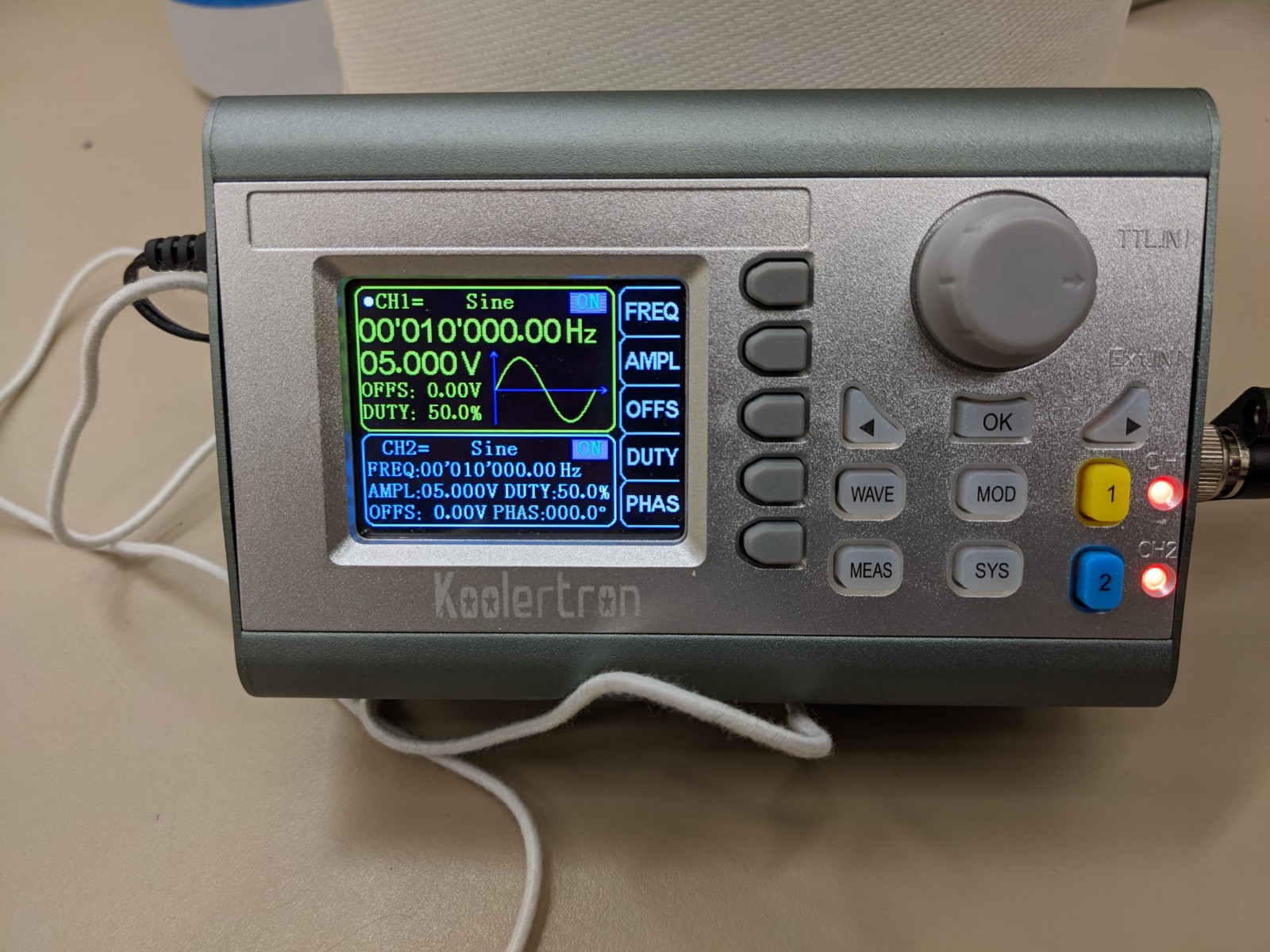
Now, attach the function generator to the wave driver. To do this, use a red banana cable to connect the red terminal on Channel 1 of the function generator to one of the banana jacks on the wave drive. Use a black banana cable to connect the black terminal of Channel 1 to the other banana jack on the wave drive. Turn the function generator On (sliding switch on the side of the unit). It will put itself in default settings. To change these to what we want:

Press the blue button 2 to select Channel 2. Press the blue button 2 again to turn output 2 Off. We are not using it.
Press the yellow button 1 to select Channel 1. Press the top gray button to choose Frequency. The knob now controls Frequency; the two arrow keys choose which digit the knob adjusts. Set the Frequency to ~30 Hertz (Hz).
Press the second gray button to select Amplitude. Use the knob to set the amplitude to 20 Volts.
Press the top gray button (again!) to select Frequency.

Part II Preliminary: Instek AFG-2005 Version

Now, attach the function generator to the wave driver. To do this, use a red banana cable to connect the red banana jack of Main on the function generator to one of the banana jacks on the wave drive. Use a black banana cable to connect the black terminal of Main to the other banana jack on the wave drive. Turn the function generator On (push button on the lower right). It will put itself in the most recent settings. To change these to what we want:

Ensure the function is Sine. To change this, press the gray FUNC button until a sinusiodal picture appears.
Ensure the ampliture is at its maximum. To change this, press the AMPL button and use the knob and arrows to get the largest amplitude possible.
Press the FREQ button, then use the knob and arrows to set the frequency to ~30 Hertz (Hz).
Press the oval OUTPUT button to get a signal out.

Part II: Measuring Stretchy-String Wave Velocity

Next, vary the frequency: you will see different nodal patterns appear and disappear as the drive frequency changes. Observe what values of n you can reach with $f$ between 10 and 80 Hertz. You definitely want at least four different possible n, and ideally at least seven. The data table has room for eight, so you don't need more entries than that regardless, although you're welcome to take them for better results. If you can't even get four different n , consult your TA.

Now, take the frequency back down to the value at which you found the least $n$ you can get out (ideally $n=1$. Slowly adjust, while watching the string, until you maximize the amplitude of that mode. You may wish to adjust by $0.1$ Hz to be as precise as (reasonably) possible.

Record $n$ and the freqency which gives maximum amplitude for $n$ anti-nodes.⁵

Repeat this measurement (varying the drive frequency) for a variety of $n$ - as many as you can get.

For each $f$ assign an uncertainty $\sigma f$ based on your judgement. This is not the uncertainty of $f$ from the function generator (this is very small) but, rather, is the range of $f's$ you could vary over and still be at about the maximum amplitude for that $n$.⁵

Part III: Measuring $\mu$ of the Fixed-Length String

Now, take the fixed-length (bright green) string. Weigh it and get its length $L_{total}$, then attach it to your wave driver.

Hook the string over the pulley, attach a $100g$ mass (to make it taut), adjust your wave drive position if needed, and measure $L$ and $\delta L$ again, as before.

Choose a value of $n$ to work with over this experiment - something you think you can measure easily, that was showing up consistently in the previous part. ($n=3$ usually works.) Record this $n$.

Now, we take off the 100g mass, and put a 50g mass there instead. Record this as $M$, and adjust the frequency of the function generator to make a pattern with n antinodes (n loops) and maximum amplitude. Record that set frequency. Repeat, adding 50g each time up until a total $M$ of 250g. (Neglect uncertainties in $M$ in this part.)

Analysis

Part I: Predicting Stretchy-String Wave Velocity

Calculate tension $F_T$ in the string and total used length of string $L' = L + \delta L$. Find mass density $\mu$ of the string in directly by using $ \mu= m/L' $. Find the uncertainty in $\mu$.

From tension and mass density, calculate wave velocity $v$. Propagate uncertainties.

Part II: Measuring Stretchy-String Wave Velocity

Make a plot of $f$ vs. $n$. Since we neglected all uncertainties, you don't need error bars.

From the slope and $L$, calculate wave velocity. Propagate uncertainty when you do so.

Answer the question about agreement with expectation.

Part III: Measuring $\mu$ of the Fixed-Length String

Calculate used length of string $L'$. Get mass density $\mu$ using $ \mu= m/L' $. Find the uncertainty in $\mu$.

For each frequency period $f$, calculate the corresponding frequency $f^2$. Then, make a plot of $f^2$ vs. $M$. No uncertainties are needed here, since we neglected all of them.

From the slope and appropriate other quantities, calculate mass density using information from the plot (ie, without using the mass $m$, the used length $L'$ string, or $\delta L$). Propagate uncertainties.

Answer the question about agreement with expectation.

Discussion Topics

Your TA will ask you to discuss some of the following points (they will tell you which ones):

Comparison to "Known" Quantities: The unstretched mass density of the white string is ~6g/m. The unstretched mass density of the green string is ~1.8g/m.⁶ Discuss whether your measurements make sense with these numbers.
Derivation of Equation \eqref{fnsq}: Do the algebra to show that equation \eqref{fnsq} holds.
Systemic Error: Distributed Weight: Suppose you had a large loop, and decided to account for some of the lost length by measuring the height of the loop and adding that to $\delta L$. This would do a reasonable job reducing the error in $L'$ for the fixed-length string, but there's still more issues for the stretchy string.
- What would be the tension in the part of the string in the loop? (Each string, not the total.)
- Suppose we were to model the string as a spring - i.e., the stretch is proportional to the tension. Why does your above conclusion indicate that, for the stretchy string, there is an error in $L'$ from the loop that cannot be accounted for by just adding the appropriate extra string length?

References and Tools

Guide to Uncertainty Propagation & Error Analysis (Quick Reference)

PHY133/134 Plotting Tool

Photogate Reference Document

Glossary

L : The length of string from wave driver to pulley. This is the relevant length in most general discussions of standing waves on a strong of length "L".
$ \delta L$ : The length of string from the pulley to the hanging mass.
L' : The sum of L and $ \delta L $. The is not the same as L_total.
L_total: The full length of the string, unstretched.
Extra L : The length of string from the wave driver to the support post (if needed). We neglect this length in some of our calculations.

Hovering over these bubbles will make a footnote pop up. Gray footnotes are citations and links to outside references.

Blue footnotes are discussions of general physics material that would break up the flow of explanation to include directly. These can be important subtleties, advanced material, historical asides, hints for questions, etc.

Yellow footnotes are details about experimental procedure or analysis. These can be reminders about how to use equipment, explanations of how to get good results, or clarifications on details of frequent confusion.

This is possible to show using just Newton's laws (considered on a small piece of the string), but it's pretty mathematically-ambitious (unless you know some multivariable calculus already). The first step is to derive the wave equation, which you can see, e.g., here. The second step is to show that any function $f(x-vt)$ or $g(x+vt)$ solves that equation, using the multivariable chain rule.

For a review of standing waves, see Giancoli Chapter 15, especially section 15-9. Or, see Katz Chapter 18.

For a review of how to tie a good knot, see The Farmer's Almanac or the Ashley Book of Knots. The old references are the best.

Of course, we know no string can be truly horizontal, at least in a gravitational field. But if the tension is high enough, we can assert that the string is approximately horizontal at rest. As a general rule, we neglect the vertical impact of gravity on our string (at least, at your current level).

If you're not familiar with why the string must sag, here's the argument: suppose the string is supported only at the ends. Then, the middle portion of the string will be pulled down by gravity (since it has some weight). There must be an upwards force balancing this, which must be tension from the ends of the string. But in order for the ends of the string to pull up, they must be pointed up, which means the string cannot be totally horizontal.

Note that for a stretchy string, as we deal with in this lab, the mass density can be changed by stretching the string. We can't just take the mass density when unstretched to determine the wave velocity, because that's not the mass density the string has when under tension.

This works just as well for waves that are simultaneously oscillating vertically and horizontally - just make $A$ and $B$ into vectors that oscillate in the perpendicular plane. The frequencies and wavelengths are the same.

You may wonder why we only consider these perpendicular oscillations, known as transverse waves. This is because the alternative, longitudinal waves, are negligible in loose string like this. They are important in other cases, though, like seismic waves (in an extreme case, earthquakes) propagating through the Earth.

This decomposition of a general oscillation into sinusoidal parts is known as a Fourier series. This is a key idea in a whole bunch of areas of physics, both as a practical computational tool and as a picture for theoretical understanding. (So, if you want to know how to calculate "how much" of each frequency there is in a general oscillation, "Fourier" is the keyword to Google.)

The idea is that our measurements of $f$ are very precise, so there's no uncertainty from the function generator. A fair objection would be that there is some range of frequencies over which one can observe that $n$; perhaps we should consider the maximum and minimum, so we can get an uncertainty range. That's a fair criticism, but finding all those is more effort than it's worth (we'll just let the plotting tool estimate our uncertainty).

Koolertron info at https://www.koolertron.com/ We also use model GW Instek AFG-2005.

It would be advisable (from the perspective of getting good data) to keep the "extra" string past the hole as small as possible.

Keep your loop as small as possible (but still big enough to easily hook/unhook several masses).

There's quite a bit of "looseness" in these measurements. (I.e.: it's not clear exactly where you're supposed to measure from/to; we're not being all that precise.) Take this into account when estimating your uncertainties.

Hopefully, your mass will not be oscillating too much. You may find that it inevitably oscillates somewhat, though (especially depending on the $n$).

We often use different fixed-length string in different rooms. (White string is most typical, but orange string is also sometimes used.) They all should lie in this range, though.