
Projectile Motion
In this lab, we will measure the horizontal distance which a projectile travels after being launched with an initial horizontal velocity.
Through these measurements and an understanding of projectile motion, we will calculate the value of \(g\), the acceleration due to gravity.
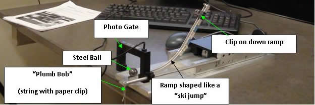
- 1 Projectile Motion Setup:
- Ramp, clamped to lab bench
- Metal ball
- Plumb bob (paper clip with string)
- Binder clip
- 1 Photogate setup
- Photogate
- Interface box ("LabPro")
- Computer
- 1 Sheet Carbon Paper, some White Paper
- 1 Meter Stick
- Record data in this Google Sheets data table
Suppose we launch an object horizontally from a height \(h\) with a horizontal velocity \(v_x\).1 The two components of motion are described by the following pair of equations:
$$x(t)=v_xt\label{xmotion}$$ $$y(t)=h-\frac{1}{2}gt^2\label{ymotion}$$Note, in particular, that the fall time \(T\) (found by setting \(y(T)=0\) is independent of the velocity \(v_x\), and is given by the equation:
$$T=\sqrt{\frac{2h}{g}}$$Plugging this back into equation \eqref{xmotion}, we therefore get the equation:
$$x(T)=v_x\sqrt{\frac{2h}{g}}$$Part I: Setting Up the Apparatus
Place your ramp so that the front edge of the platform lines up with the edge of the table (so that when the ball rolls off the ramp, it goes straight off the edge). Clamp it down so that the position is fixed.
Hang the paper clip from the end of the ramp. Ensure that it is not resting on the floor, but instead hanging a short distance (a cm or two) above it. This gives you a purely-vertical line from the bottom of the ramp to the floor directly below (which will allow us to measure horizontal distance precisely). This setup of having a hanging mass to show you a vertical line is called a plumb bob.
Place the ball right at the end of the ramp (you may have to hold it there). Measure the distance \(h\) vertically from the bottom of the ball to the floor, using your plumb bob as a guide to a perfect vertical. Estimate an uncertainty in this distance \(h\) as well.
Next, set up your photogate. Mount it onto the stand at the side of the ramp, and ensure that the beam crosses that track at approximately the center of the ball when the ball is placed at the relevant position. Plug it into "DIG/SONIC 1" port of the "LabPro" on the wall.
On the computer, find the folder with LoggerPro files. Open "Projectile Motion"; click "Connect" on the box that pops up.
Click the green "Start Collection" button at the top of the screen to start "recording" the output of the photogate. Roll the ball down the hill and ensure that it shows two times: one at which the ball entered the photogate, and one at which the ball left it.
If so, press "Stop Collection" (same button)1 - everything is set up correctly, and you can move on to the next part. If not, consult your TA.
Part II: Determining the Effective Diameter of the Steel Ball
We are going to determine the velocity by measuring the time \(\delta t\) it takes the ball to cross in front of the photogate.
Velocity is change in position over change in time, so we need to determine first how far the ball will move when it crosses the photogate.
If the photogate were exactly halfway down the ball, then this distance would be the diameter of the ball. However, we cannot rely on that assumption.
Instead, we will measure the effective diameter, \(d_\text{eff}\), of the ball, which is the length of the chord that actually passes by the photogate.
To do this, we will use the screw on the base of the platform, which will slowly move the photogate back and forth.2
Each turn of the screw will move the photogate some known distance. Therefore, we will determine how many turns of the screw it takes for the photogate to move across the ball, and thereby determine the effective diameter.
First, take note of the pitch of the screw. This is the distance the photogate will travel per turn. Depending on your platform, this may be 1mm or 1/28" (which is approximately 0.907mm). Record this distance on your data sheet (there is a drop-down).
Then, turn the screw until the photogate beam is a few turns past the end of your ball.3
Now, turn back the other way, slowly. Once the photogate turns from "unblocked" (light off) to "blocked" (light on), start counting the number of turns. Count until it reads "unblocked" (light off) again. This is how many turns it took the photogate to pass your ball.
Estimate an uncertainty in how many turns it took to complete this process, as well. (Is a quarter-turn reasonable? More? Less?)
Multiply the number of turns by the pitch of the screw to get your effective diameter. (Multiply the uncertainty in number of turns by the pitch to get the uncertainty in effective diameter.)
If your effective diameter is less than 5mm, your photogate is too close to the top or bottom of the ball for good results - reposition it (higher or lower, depending on where it's striking the ball) and try again. Otherwise, don't let your photogate move from this point forward in the experiment, or you'll have to restart!4
Part III: Using Projectile Motion to Measure \(g\)
Now that we're finally done with the preliminary stages, it's time to let things fly!
Attach the binder clip so that the bottom of the binder clip is just above the "curve" on the incline.5 Place the ball just below the binder clip so that the top of the ball is resting against the bottom of the binder clip.
Release the ball and see where it lands. Place a sheet of white paper on that location and the carbon paper on top (dark side down). When the ball lands on the carbon paper, it will leave a small circular mark.
(Ensure that the white paper is clean enough to see where the ball lands - if there are markings from a previous set of drops, make sure that they are at least x-ed out so that you can know which ones are the new ones!)
Tape down the white paper to ensure it does not move. Do not tape down the carbon paper.6
Press the green button "Start Collection" button on the computer screen again to begin your first data set. (Give the computer a second or two to actually start collecting.) Align the ball with the bottom of the binder clip as before, and release.
It should roll through the photogate and land on the carbon paper, recording two times on the computer and making a mark on the white paper. If you get fewer than two times from the photogate, you probably let go too soon - cross out the mark left on the white paper, and repeat the trial.
Assuming it worked: first, take note of the difference between the two times on the computer. This will be \(\delta t\) for this trial (trial 1 of the lowest position).
Then, lift the carbon paper and measure the horizontal distance from the bottom of the plumb bob (the paper clip) to the center of the mark left on the paper. This will be the distance \(x\) travelled by the ball (which we call \(x(T)\) above).
Cross out the mark that the ball made, so you know you already measured that spot. Place the carbon sheet back down again and click "Stop Collection."
Then, place the ball back on the ramp at the same position (do not move the binder clip!) and repeat your data collection for two more trials. If at any point the ball lands off the paper (it shouldn't if you have positioned things correctly), remove all data for that set of trials, reposition the paper better, and try again.
Finally, repeat everything you just did in this part for four higher positions on the ramp (moving the binder clip up each time). You should reposition the paper and take three trials each time. If your paper sheet gets too messy to see new marks, flip it over; if that side is also too heavily marked, get another one.
The only thing that will be different is that for your last trial, you can disregard the binder clip altogether. There is a small metal peg at the top of the ramp, and you can rest the ball against the bottom of that instead of the bottom of the binder clip.
Once you have taken three points of data for five different heights, you have all the data you need!
If you think you might have bumped your photogate at any point during this process, you should quickly repeat part II to ensure that the photogate hasn't moved. If you get a significantly different \(d_\text{eff}\), you probably bumped something during the experiments, which will throw off your results, in which case you'll need to retake your data - you can't trust the velocity measurements at that point.
For each ramp height, compute the average \(x\) distance travelled, \(x_\text{avg}\), and average time taken to pass through the photogate, \(\delta t_\text{avg}\). Also compute the uncertainty in these averages.
From \(\delta t_\text{avg}\) and the effective diameter of the ball \(d_\text{eff}\), calculate the horizontal velocity for each ramp height, \(v_x\), using \(v_x=d_\text{eff}/\delta t_\text{avg}\). Propagate uncertainty into \(v_x\).
Make a plot of \(x_\text{avg}\) vs. \(v_x\). Identify the units on your slope (note: these may need to be simplified, depending on your units of \(v_x\) and \(x\)).
From your slope, calculate \(g\). Propagate uncertainties as well.7 Finally, state whether your calculation of \(g\) agreed with the expected value.
Your TA will ask you to discuss some of the following points (they will tell you which ones):
- Comparing Random Errors: Compare your different sources of random error. What do you think contributes most to your uncertainty in \(g\)? Make your comparisons quantitatively.1
- Friction: Friction on the ramp might slow the ball as it rolls down the hill. Discuss the impact of this as a systemic error - in particular, what would be the impact on \(g\)? Note that there's an important subtlety here to discuss: friction before the photogate and friction after the photogate act differently as systemic errors. How and why?
- Launch Angle: Although these setups are designed to launch the ball horizontally, they may not do so perfectly. They may, in fact, launch the ball at a slight upwards or downwards angle. Discuss the impacts of this systemic error: how would the range depend on the angle? (Does the effect depend on \(h\), \(g\), and/or \(v\)?)
- Rolling Off (Dimensional Analysis): Clearly, at very low speeds, something happens that is not what we expect: the ball travels a minimum distance of \(R\), the radius of the ball. This is because it rolls off the edge, rather than the presumed abrupt disappearance of the table holding it up. This is a rather complicated issue to solve exactly; nevertheless, with a bit more physics, it is possible to deduce that this is not a problem once you exceed a minimum velocity \(v_\text{min}\) of rolling off the table.2 Consider what parameters of the problem are relevant (\(R\), \(g\), \(h\), etc.) and, using dimensional analysis, get an order-of-magnitude estimate for \(v_\text{min}\) (which happens, if you don't include any extra factors, to be exact). How does this estimate compare to the measured velocities in your data - is this a concerning systemic error?
- Air Resistance: A simple model for air resistance estimates the force on an object due to air resistance as: $$F=\frac{1}{2}C\rho_\text{air} v^2 A$$ Here, \(C\) is the drag coefficient (0.47 for a sphere), \(\rho_\text{air}\) is the density of air (which you can look up), \(v\) is the velocity of the object (relative to the air), and \(A\) is the cross-sectional area of the object. By contrast, the gravitational force on the ball is \(F=mg\). Compare these two forces, making reasonable estimate for \(m\) and \(A\) and using a typical value for \(v\) based on your data: how relevant is air resistance as a systemic error in this lab?
Hovering over these bubbles will make a footnote pop up. Gray footnotes are citations and links to outside references.
Blue footnotes are discussions of general physics material that would break up the flow of explanation to include directly. These can be important subtleties, advanced material, historical asides, hints for questions, etc.
Yellow footnotes are details about experimental procedure or analysis. These can be reminders about how to use equipment, explanations of how to get good results, or clarifications on details of frequent confusion.
For details on projectile motion, see Katz Ch. 4 or Giancoli Ch. 3
The software will automatically stop recording after some span of time. Once it says "Start Collection" again, it's already stopped, so you don't need to stop it (and in fact, you will overwrite your previous data if you click "Start Collection" again).
This will be more precise than just using the length scale on the platform.
There is a phenomenon in screws known as "backlash," where the screws will be a little loose when you reverse directions of rotation, meaning that the photogate won't move at first. You want to be sure to be past this point by the time you are beginning your measurements.
If you bump it higher or lower, you will change how high the photogate beam will be on the ball. This will change the length of the horizontal chord across the ball, which is what we call \(d_\text{eff}\) - and all the rest of your measurements are reliant on knowing your value for \(d_\text{eff}\)!
The idea is to place it close to the bottom of the ramp, but still high enough that the ball will pick up some speed.
We don't really care how the carbon paper moves, so long as it stays on top of the white paper, and the tape tends to tear the carbon paper when taken off (and we want to be able to reuse it).
This propagation is complicated, and so is broken into steps on the data table for your convenience.
Hint: is relative or absolute error more suited to discussing errors from different sources, with potentially different units?
This can be derived by showing that, for it to roll off slowly rather than flying off, the downward force must be at least equal to the centripetal force as it rolls over the edge.