Pendulum

In this lab, we determine how the period of a pendulum (time for one full oscillation back and forth) depends on the length of the pendulum and how much the pendulum swings.Hoveroverthese!
Through these measurements and a theoretical formula that pendula should follow, we will calculate the value of \(g\), the acceleration due to gravity.
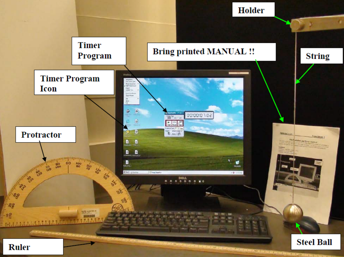
- 1 Pendulum Setup (Metal Bars, String, Steel Ball)
- 1 Protractor
- 1 Meter Stick
- 1 Stopwatch (feel free to use your phone, or just Google "stopwatch" and use the one that comes up)
- Record data in this Google Sheets data table
Although pendula come much later in the physics curriculum than the material you have covered so far,1 you almost assuredly have experience with a pendulum of some form from your everyday experience. They swing back and forth periodically, from some maximum angle to the opposite side and back again.
For sake of physical simplicity, we assume that the pendulum is "rigid" (is of fixed shape and size as it oscillates) and that the top of the pendulum is fixed (so it's swinging from a single point). We also typically assume that the pendulum is planar (swings in only the \(xy\) plane with no \(z\) motion), although with the approximations we will make in this lab, that assumption is not strictly necessary.
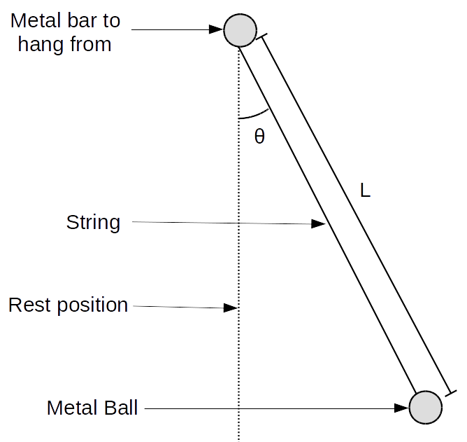
The simplest picture of a pendulum is called, appropriately, a simple pendulum. This consists of a very small object hanging from a long essentially-massless string. The approximations we make are that the size of the object is much smaller than the length of the string and that the object is much heavier than the string.
Under these approximations, a pendulum of length \(L\) (measured to the center of the hanging object) looks as follows:

In this lab, we are interested in the period, \(T\), of the pendulum. This is the time it takes the pendulum to complete one full swing - from one side to the other and back again (or, equivalently, from the middle, up to one side, down past the middle and up the other side, and back down to the middle again).
When oscillations are small (i.e., the pendulum isn't swinging too much),1 we can make a small angle approximation which allows us to derive the following simple formula for the period of a simple pendulum of length \(L\) in a gravitational field of strength \(g\):
$$T=2\pi\sqrt{\frac{L}{g}}\label{SmallAngleT}$$When oscillations are large, we expect the period to deviate from this simple formula.2
Part I: Determining the Random Error in Time Measurements
Before we start measuring periods of oscillations and trying to validate the above formula, let's understand the uncertainty in our measurements.
While we can reasonably estimate an uncertainty in our length measurement, it's not immediately obvious how precisely we can measure the period of the pendulum.
The stopwatch on the computer measures to a hundredth of a second, but we should be careful: our measurements are hardly that precise. The dominant source of uncertainty here is from your hand, not the computer - and who knows what that uncertainty is? It probably varies from person to person! Thus, we have to measure it.
Set the length of the pendulum to 50cm or so.1 You don't have to be precise with the length yet; we're not concerned about the actual values.
Have one partner (Partner 1) hold the stopwatch, and the other partner (Partner 2) hold the pendulum up at a small angle from the vertical (say, \(15^\circ\) or so - again, no need to be precise yet).
Have Partner 2 release the pendulum and let it swing. After a swing or two, Partner 1 should hit the start button at the bottom of the swing.
Time how long it takes the pendulum to complete ten swings back and forth.23
Record the time to undergo ten swings in your data table as Trial 1. Repeat this procedure for four more trials.
Then, swap partner positions, and record five trials with the other partner timing.
Part II: Determining the Dependence of Period on Angle \(\theta\)
Now, we're going to do the same measurement - time for ten swings - for different angles. Leave the length as it is.
As before, have one partner operate the stopwatch and the other measure the angle and start the swinging. (Remember who held the stopwatch - you'll want to use their uncertainty in period.)
Begin with a \(15^\circ\) angle from the vertical.4
Release (be careful to give it as little initial velocity as possible!), and measure ten periods. Record this on your data table.
Repeat for angles \(30^\circ\) and \(80^\circ\) from the vertical.
Part III: Determining the Dependence of Period on Pendulum Length \(L\) and Measuring \(g\)
Again, same measurement, just varying length this time.
Begin by setting the length to 10cm or so. Measure this length from the point where the pendulum swings (the top of the string) to the center of the ball (to the best of your ability to estimate the center of the ball).
Estimate your uncertainty in your measurement of this length. This requires some thought: what is your dominant uncertainty here?3
At this length, measure ten periods at \(15^\circ\), same as before.
Repeat this measurement for lengths increasing to about 1m in increments of about 10cm, measuring the actual length L (which may not be exactly 10cm, 20cm, etc.!) with your meter stick each time.
Part I: Determining the Random Error in Time Measurements
For each partner, calculate the mean of all five measurements. Then, calculate the uncertainty in the mean of these measurements and the uncertainty of an individual measurement.
Then, answer the question on the data table, using the appropriate uncertainty for the comparison you are doing.
Part II: Determining the Dependence of Period on Angle \(\theta\)
For each angle, take the uncertainty in \(10T\) to be given by your uncertainty from Part I. (Think: which one should you use?)
Calculate the period \(T\) for each angle. Propagate uncertainty from \(10T\) to \(T\). Then, answer the questions on the data table. about these period measurements.
Part III: Determining the Dependence of Period on Pendulum Length \(L\) and Measuring \(g\)
Take the uncertainty in \(10T\) as from Part I, and calculate the period \(T\) and the uncertainty in \(T\) (just as you did for Part II).
Calculate \(T^2\) and \(L^2\). Propagate uncertainties from \(T\) and \(L\) into uncertainties in these quantities.
Make three plots: one of \(L\) vs. \(T\), one of \(L^2\) vs. \(T\), and one of \(L\) vs. \(T^2\) using the PHY133/134 Plotting Tool. For each of these plots, you should include error bars on each axis (equal to your calculated uncertainties in the relevant quantities), good axis labels, and a good title. See the Guide to Making and Using Plots, as well as the Lab Report Expectations for more details.
Take the slope of the most linear graph, and enter it into your data table. From this slope, calculate \(g\), and propagate uncertainty from slope to \(g\). (If you are confused by how to get \(g\) from the slope, see the last section of the Guide to Making and Using Plots - you'll have to rearrange formula \eqref{SmallAngleT}.)
Finally, answer the question on the data table for this part.
Your TA will ask you to discuss some of the following points (they will tell you which ones):
- Kinds of Error in Period: In Part I, you made a comparison between each partner's timing of the same pendulum under the same conditions. Some kinds of uncertainty are included in the uncertainty you used to make this comparison, some kinds are not included in the uncertainty and will cause a discrepancy between you and your partner, and some kinds are not included in the uncertainty. and will affect you and your partner identically.4 Give examples of what kinds of errors would fall into these different cases. (Hint: some things vary from trial to trial; some things vary from partner to partner; and some things are consistent between you and your partner's setups.) Then, discuss what your specific results tell you about these different uncertainties.
- Uncertainty in Length: What did you consider to be the dominant source of uncertainty when measuring \(L\)? Why did you pick the uncertainty that you did?
- Procedure: Measuring Period: Why might measuring the time at the bottom of the swing yield better precision than measuring at one end?5
- Quantitative Estimate of \(L\) Dependence of \(T\): One way to quantitatively determine the dependence of \(T\) on \(L\) (i.e., specifically determine that it's a square root) is to make a plot of \(\ln(T)\) vs. \(\ln(L)\). Make this plot using your Part III data (ignore units for your axis labels; that's a complicated discussion that's not important for what we're doing).6 Based on equation \(\eqref{SmallAngleT}\), what should the slope of this plot be? Does the slope of your plot agree with what you expect? (This is a better way of doing what we did by making three plots and choosing the most linear one.)
- Systemic Error: Massive String: We made an idealization that the string was massless. Suppose the string in fact had a significant mass. Would you expect the period to increase or decrease, and why? (Hint: you can qualitatively treat the mass of the string as reducing the "average" length of the pendulum.)
- Quantitative Systemic Error: We made two key assumptions in calling our system a "simple pendulum": a massless string, and a small-sized hanging object. Although you don't have the physics knowledge to calculate the impacts of violating these assumptions exactly, you can still estimate the order of magnitude of the impacts by estimating the relative size of these quantities. Estimate quantitatively how the mass of the string compares to the mass of the hanging object, and how the radius of the object compares to the length of the string. To an (admittedly very rough) approximation7, this will (usually) be the order of magnitude of the errors induced by these quantities not being exactly zero. Consider the relative errors you just calculated: how important are these errors? Which is more important (i.e., if we wanted to "improve" this experiment, which would be the more important one to improve)?
- Dimensional Analysis: Often, we can almost derive formulas (up to an overall constant) just by knowing the units of the relevant quantities. Under the assumption that the pendulum's period can only depend on the pendulum's length \(L\), mass \(m\), maximum angle \(\theta\), and the strength of gravity \(g\) (with units \([g]\)=m/s2), explain why we must have a relation like \(T=f(\theta)\times\sqrt{\frac{L}{g}}\).2 (Note that \(\theta\) counts as a unitless parameter here.) Asserting \(f(\theta)\simeq f(0)\) in this formula is the small angle approximation (where \(f(0)=2\pi\) is found by other means).
- Small Angle Approximation: The approximation that leads us to formula \eqref{SmallAngleT} is that \(\sin(\theta)\simeq\theta\) for small \(\theta\) (where \(\theta\) denotes the maximum angle of swing, in radians). Compare \(\sin(\theta)\) and \(\theta\) for each of the angles we used in Part II: how much do they differ? Take the relative difference between those two quantities as a rough estimate of the deviation of the pendulum from what you expect; how precise is that formula in each case? For how large of an angle is the formula useful?
- Exact Planar Pendulum Solution: The full general formula for the period of a planar pendulum of arbitrary amplitude is: $$T=T_0\times\frac{2}{\pi}K(\sin(\theta/2))$$ where \(T_0\) is the period from our small angle approximation, \(\theta\) is the maximum angle the pendulum swings, and \(K\) is a special function called the complete elliptic integral of the first kind.3 Using a program like Wolfram|Alpha,5 calculate the correction factor \(\frac{2}{\pi}K(\sin(\theta/2))\) for each of the angles you measure in part II.6 How big is the correction (i.e., how far is this number from 1)? Does the period get bigger or smaller for large angles? How does the theoretical deviation from expectation compare to your results in Part 2?
Guide to Uncertainty Propagation & Error Analysis Quick Reference for Uncertainties
Hovering over these bubbles will make a footnote pop up. Gray footnotes are citations and links to outside references.
Blue footnotes are discussions of general physics material that would break up the flow of explanation to include directly. These can be important subtleties, advanced material, historical asides, hints for questions, etc.
Yellow footnotes are details about experimental procedure or analysis. These can be reminders about how to use equipment, explanations of how to get good results, troubleshooting tips, or clarifications on details of frequent confusion.
To read ahead in your textbook and get more detail, see Giancoli 4th ed. ch. 14-5 or Katz ch. 16-6.
Formally, this follows from the Buckingham Pi Theorem, which extends Rayleigh's method of dimensional analysis.
For more details on this function, see here. For the derivation of this formula from first principles, see here.
To be more quantitative: we are approximating that \(\sin(\theta)\simeq\theta\), so the approximation we make is valid when that approximation is valid.
In the planar case, one can find an explicit formula for the period of a pendulum in terms of elliptic integrals, but that's beyond the scope of what we're doing here.
In particular, which is most important: the precision in reading the ruler itself, your ability to estimate the location of the center of mass of the hanging object, or your ability to estimate the location of the swing point? (Or are multiple of these large enough to be important?)
The first kind of errors are not necessarily worrisome - while we would like to reduce them to increase precision, if they are large, our results will be compatible because our self-described uncertainties would be large.
The second kind of errors are worrisome, because we don't include them in our uncertainty, so we may measure a discrepancy due to this kind of error that is not a "real" discrepancy and should be accommodated by our "true" uncertainty (which would include these factors). Thus, running this kind of check is important, to detect those!
The third kind of errors is even worse - the check we ran didn't account for it, and so we have virtually no understanding of whether that kind of error is important, experimentally-speaking!
Hint: what is the quantity we are measuring (for which we want to minimize uncertainty)? If the speed is higher, what does this do to our uncertainty in that quantity, and why?
Technically, the argument of \(\ln\) should be unitless, so what we're doing is taking the log of \(\frac{T}{1\text{s}}\) and \(\frac{L}{1\text{m}}\) (or whatever unit you chose to measure in). These units don't matter, however, since the difference between units is multiplicative inside the logarithm, and therefore additive outside of it, so all of this dependence goes into the intercept. Since we'll only be interested in the slope here, we won't concern ourselves with those details.
Formally, if you have some calculus background: you can take whatever the "fully correct" solution is, and make a Taylor expansion in the appropriate "small" (dimensionless) quantity; for instance, the ratio of mass of string to mass of hanging object. If our solution is the zeroth-order expansion, we can consider the first-order expansion, and get that relative error times some derivative term (which we assume to be of order of magnitude 1).
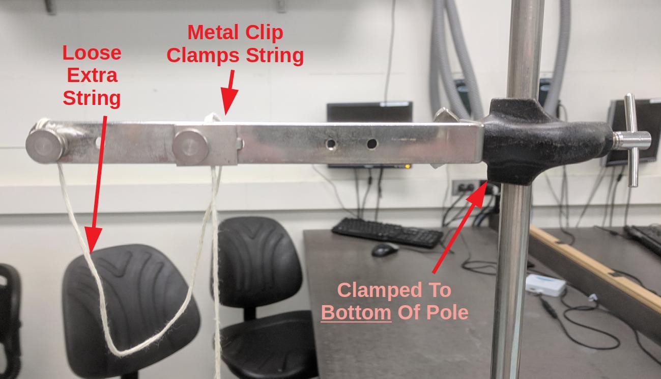
Ideally, your setup should look like this:

in which case you should be able to slide your string freely by loosinging the screw a bit, then clamp it at any height. Your clamp may be on the outside instead; that's fine. If you are missing the metal clamp entirely, wind/unwind the rope around the screws to change length instead.
For optimal results, count when it is at the bottom of its swing. This maximizes your timing precision in determining the period. (If you don't believe this, feel free to test, and compare the uncertainty of the two methods yourself!)
A convenient way to count (to make sure that you don't end up making a mistake) is to, when you press the start button, say "zero." Then, as it swings back and forth past the bottom, count: "zero, and, one, and, two..." Then, stop when you say "ten."
Keep in mind how to properly use a protractor (measure the angle from the appropriate point on the protractor).
You should just be able to enter "K" and the computer will understand what you mean; if not, try "EllipticK" instead.
Note Wolfram|Alpha assumes angles are entered in radians by default, although if you say "sin(90 degrees)" explicitly then it will give you the correct results.