Conservation of Energy

In this lab, we will study the principle of conservation of energy as gravitational potential energy is converted into kinetic energy.
- 1 Air Track Setup
- 1 Air Track (attached to air pump)
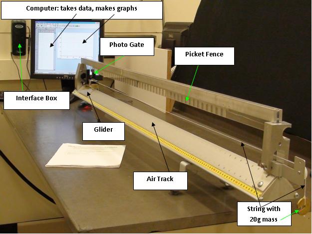
- 1 Cart w/ Photogate
- 1 Picket Fence
- 2x 20g Mass
- 1 Meter Stick
- 1 Scale (or, access to one of several shared with room)
- Record data in this Google Sheets data table
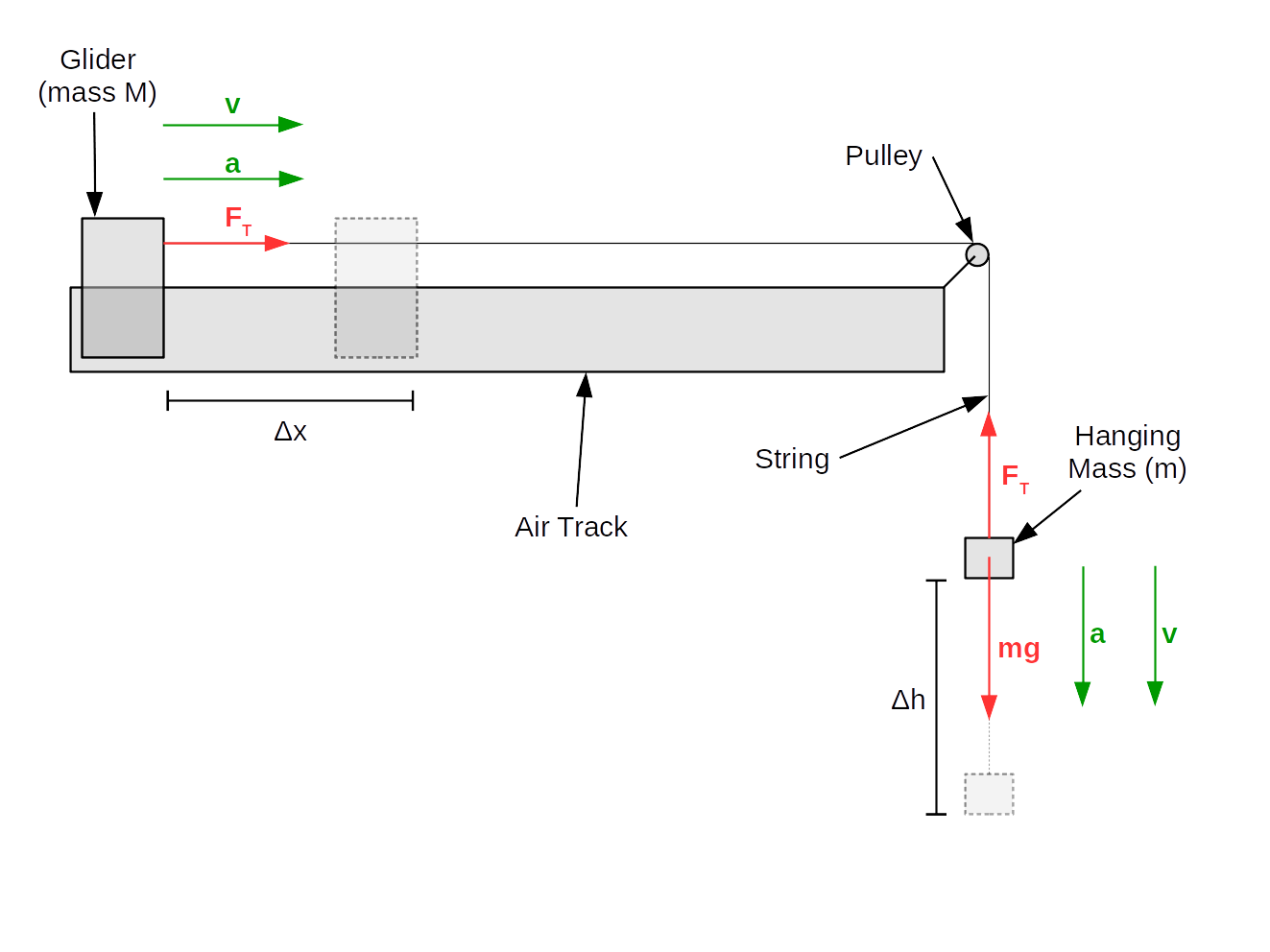
In this lab, we will have a mass attached to a string that hangs over a (massless, frictionless) pulley. The other end of the string is attached to a cart on an air track. An air track is like a one-dimensional air-hockey table: it ejects air in order to minimize friction.
In maintaining a nearly frictionless environment, we have isolated our system (to a high degree of precision), meaning energy will be conserved.1
Schematically, the system is hooked up as follows:

Recall that \(PE=mgh\), so \(\Delta PE=mg\Delta h\). Noting that \(\Delta h=-\Delta x\), we have:
$$\Delta PE=-mg\Delta x$$Or, more concisely, since "zero potential energy" is arbitrary, we simply assert:
$$PE=-mgx$$For kinetic energy, we have simply:
$$KE=\frac{1}{2}mv^2+\frac{1}{2}Mv^2=\frac{1}{2}(m+M)v^2$$The law of conservation of energy states that:
$$\frac{dE_\text{total}}{dt}=0\label{ConsEn}$$Here and in general, \(E_{total}=KE+PE\) (although the expressions for those quantities will vary from system to system).2
Click here for modifications to directions if you are in room A118.
Because you we don't have enough "rail and mounted photogate" setups for everyone, you get an ultra pulley to measure distance instead. This induces the following modifications to the procedure:
- Take \(D\) to be 15cm,Source with \(N\) as 10 (for the 10 spokes).
- To approximate your uncertainty in \(D\), take the thickness of your string (nominally, an uncertainty in radius) and multiply it by \(2\pi\) (to convert to an uncertainty in circumference). Feel free to round off this uncertainty as you see fit.
- Neglect instructions about measuring \(D\) yourself. Calculate \(d\) in the same way as usual.
Part I: Preliminary Setup and Measurements
Once your TA turns on the air, begin by leveling your air track. Place the cart in the middle of the track, and make sure it doesn't slide to the left or right. If it does, turn the screw on the leg of the air track to adjust the height until the air track is level (in the center).3
Similar to how we did in the acceleration lab, we need to set a scale for the photogate. Measure \(D\), the length of some number of black-clear segments (say, 10), and divide by the number of segments to get \(d\), the length of one segment.1
Open "ConservationofEnergy" and ensure your photogate is connected correctly.4
Weigh your glider2 to get the mass \(M\). Identify the two masses \(m\) you'll be hanging from the bottom of your string. Take an uncertainty in \(M\) based on the last decimal place of your scale, and in \(m\) of 0.1g (for both parts).5
Hook a string from the glider over the pulley at the end of the air track and down. Ensure that the cart has plenty of space to move before the mass hits the floor.
Part II: Using a 20g Mass
Hook the 20g mass up to the bottom of the string, and pull the cart to the end of the track opposite the pulley.
Press "Start Collection," wait a second, and release the mass. Catch the cart before it reaches the other side, and press "Stop Collection."
Highlight the region of the velocity vs. time plot which is a straight line, and identify which data points that corresponds to.
From the data table, record the time, position and velocity values for the first ten data points of that region. If the region is not long enough, repeat the experiment.
Part III: Using two 20g Masses
Do everything you did in the previous part, except this time with 40g (two 20g masses) instead of 20g hanging off the string.
For each mass, do the following:
- Calculate the weight of the hanging mass, \(F_g\), and the total mass \(m+M\). Propagate uncertainties.
- Convert position and velocity to "physical" units using \(d\). Propagate uncertainty (from \(d\)).
- Calculate \(v^2\) and propagate uncertainty (as a useful middle step).
- Calculate PE and KE at each time. Add them together to get \(E_\text{total}\). Propagate uncertainty.
- Make a plot of total energy vs. time (with error bars on energy). Note your slope, and compare it with expectation.
If you use Google Sheets efficiently, repeating for many measurements across two parts shouldn't require much modification.
Your TA will ask you to discuss some of the following points (they will tell you which ones):
- Deriving Conservation of Energy: Suppose we have a single particle moving in one dimension whose potential energy as a function of \(x\) is \(U(x)\). Show (using the chain rule and the relationship \(F(x)=-U'(x)\)) equation \eqref{ConsEn}, Conservation of Energy, for this system.
- Systemic Errors
- Friction: We assumed the pulley is frictionless. If not, what would be the impact on our energy vs. time plot?
- Massive Pulley: We assumed the pulley is massless. In reality, it has some mass, which means it has some kinetic energy (and, presumably, this kinetic energy increases as you go faster).1 Since the pulley does in fact have some mass, what impact would this have on the slope of our energy vs. time plot?
- Inverse Process: Suppose instead of dropping the mass, we had started with the mass moving up (from an initial push), and recorded until it stopped. How would this change how each of those systemic errors manifest (if at all)?
- Data Visualization: An alternative (equally-viable) way to picture this data is to make a PE vs. KE plot.
- Expectation: Make the plot. What is the expectation for the data according to conservation of energy? (Is it the slope, the intercept, or a combination of both that you use determine conservation of energy, and how so?) Does your data match this?
- Systemic Errors: Consider the two systemic errors mentioned above (friction and the massive pulley). How would these manifest on this plot?
- Strengths/Weaknesses: For which plot (PE vs. KE or energy vs. time) can you understand the effects of friction without knowing the details of the experiment? What about the mass of the pulley? (Hint: how do the manifestations of these errors change if we run the "inverse process" mentioned above?)
- Acceleration: Derive a formula for acceleration of the system in this lab (under the assumption that the pulley is massless and frictionless, so the two tension forces are equal). How could one use this formula (similar to the Atwoods machine) to get a measurement of \(g\)?
Hovering over these bubbles will make a footnote pop up. Gray footnotes are citations and links to outside references.
Blue footnotes are discussions of general physics material that would break up the flow of explanation to include directly. These can be important subtleties, advanced material, historical asides, hints for questions, etc.
Yellow footnotes are details about experimental procedure or analysis. These can be reminders about how to use equipment, explanations of how to get good results, troubleshooting tips, or clarifications on details of frequent confusion.
For an overview of Conservation of Energy, see Chapter 8 of either Katz or Giancoli
The texts Katz and Giancoli use E for Total Energy, U for Potential Energy and K for Kinetic Energy.
For more details, see our Air Track Reference Document.
For more details, see the Photogate Reference Document, although hopefully you know how to do it by now.
\(m\) uncertainties taken (approximately) from here
This information taken from the User Manual for this pulley.
These and other measurements that are common between both data tables will automatically copy from the top table to the bottom one.
You will have to take the top part off the track to get your cart off the track, then put it back on later.
In fact, if the shape of the object spinning is fixed, kinetic energy is proportional to the square of the tangent velocity at some fixed radius (where "tangent velocity at some fixed radius" is what we measured in this lab).