In this lab, we will study one-dimensional kinematics under constant acceleration.

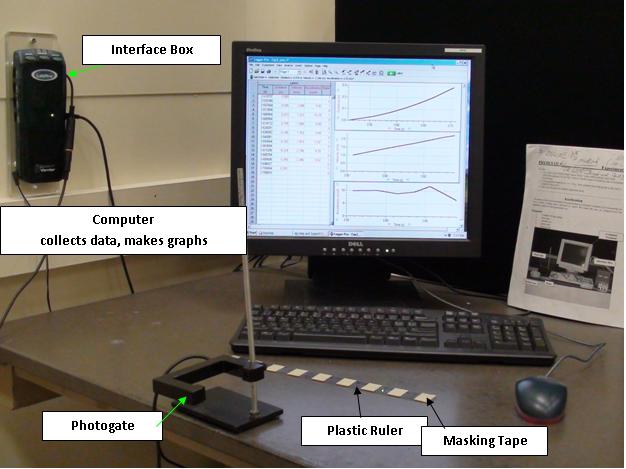
We will measure the rate of acceleration, which will be the acceleration due to gravity, \(g\).^{Hoveroverthese!}

• 1 Vernier Picket Fence
• 1 Photogate setup
  • Photogate
  • Interface box ("LabPro")
  • Computer
• Record data in this Google Sheets data table

The primary fact we will be using in part I is that the slope of a velocity vs. time graph is acceleration.¹

In part II, we will be using the kinematic equation (in the vertical direction):

$$v_{yf}^2=v_{y0}^2+2a\Delta y$$

Procedurally speaking, we will be performing this lab using a Photogate.

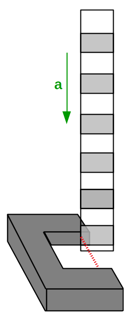
This device has an LED and a light detector that is able to "see" that LED light precisely when there is nothing in the way of the beam. In this way, it is able to see whether the beam is "blocked" or "unblocked," and measure the times at which this changes.

In this lab, we will be dropping a "picket fence" with black and clear stripes at regular intervals through the photogate, as follows:

By measuring the length of these strips, we know how far it has fallen whenever it switches from "blocked" to "unblocked" or vice versa. Thus, we will know the y-position at various times, enabling us to understand the kinematics of our system.

Part I: Measuring \(g\) Using a Velocity Vs. Time Graph

First, take your striped plastic rectangle, and measure the distance \(D\) between the bottom of the lowest black stripe and the bottom of the highest black stripe. Estimate your uncertainty in this measurement. Also record how many segments (pairs of black and white stripes) this is as \(N\).

Turn on the lab computer and log in as "Student" (if necessary). Open the file "Acceleration" from the LoggerPro file folder on the computer. In the window that pops up, click "Connect." This should set up the photogate with the computer.¹

At this point, you should be confronted with a screen with three plots on the right and a data table on the left.²

Make sure the photogate is mounted over the floor such that the striped plastic can fall through it when dropped. It may be convenient to put a chair underneath to catch the picket fence (but low enough so that the fence passes all the way through and does not bounce back "in sight" of the photogate).

Hold the fence just above the photogate, oriented so that the black and white stripes will go across the beam and block it (i.e., in the plane perpendicular to the laser beam). Make sure that the photogate starts out unblocked, so you are holding it high enough.

Press "Start Collection," wait a second for it to register, and when it actually begins collecting data, drop the fence through. Make sure the fence drops straight through and does not rotate (be careful how you drop it), and also that it does not hit the photogate on the way down.

Once it is through, press "Stop Collection." You should see some data and three plots: a position vs. time plot, a velocity vs. time plot, and an acceleration vs. time plot, all with distance units of "segments" (pairs of black/white stripes).

Look at these plots. Do they look like what you expect?³

If there is a kink in the plot somewhere (it does not look how you expect), if it hit the photogate, or if it rotated significantly as it dropped, take the data again (click "Start Collection" and drop it again). Also do so if you have fewer than three total velocity measurements (look to the table on the left to see how many data points you have).

If the data looks OK, then make a quick sketch of what they look like on the provided sketching paper. (You may want to take a screenshot for later reference as well.)

Fit a best fit line to your velocity vs. time plot as follows: highlight the data on the plot in the region where it looks like a straight line. (I.e., if it dropped smoothly, all of your data; if it bounced back in sight of the photogate, only the data before the bounce). Click "Analyze->Linear Fit" and it will output a fit with a slope. Record the slope of this line, and then click the "x" of the little "fit" box to close it.

Repeat the process (take data, check that it looks good, fit) for four more drops. (No need to sketch again, though.)

Part II: Measuring \(g\) Using Drops from Varying Height

Now, we will take a different set of measurements. We will hold the striped plastic some distance above the photogate, drop it, and look at the first velocity measured vs. height above the photogate dropped.

Begin by holding the plastic such that the bottom of the lowest black segment is about 2cm above the top of the photogate. Record this distance (as best you can measure it) to be the height \(h\).⁴

Take your uncertainty in height to be 2mm, which is dominated by the uncertainty in your ability to hold it at exactly 2cm, unless you think you did better than that, in which case you are welcome to make your own assessment.

As before, click "Start Collection," wait a second, and drop the fence. Take note of the first velocity the program records (the first measurement listed on the data table at left), and record it.

Repeat dropping from higher distances - 4cm, 6cm, etc. up to 10cm, noting the first velocity measured each time.

Part I: Measuring \(g\) Using a Velocity Vs. Time Graph

Take your five slopes, take an average, and calculate the uncertainty in this average.

As the slope of a velocity vs. time graph, the quantity measured was acceleration, which should be acceleration due to gravity. The units begin are a little wonky right now, though - "segments per second squared."

Let's fix that. First, divide the length of all the segments \(D\) by the number of segments \(N\) to get the length a single segment \(d\), and propagate uncertainty.

Then, to convert our measurement of \(g\), we just take the measurement in segments per second squared, and multiply by \(d\), the physical distance per segment. Propagate uncertainty, taking into account both the uncertainty in \(d\) and the uncertainty in the average slope.

Finally, state whether this value of \(g\) agrees with the accepted value of \(9.81\)m/s\(^2\).

Part II: Measuring \(g\) Using Drops from Varying Height

First, convert your measurements of \(v\) to physical units, following the same method as for \(g\): multiply by \(d\). Propagate uncertainty, this time assuming \(v\) doesn't have uncertainty.

From there, calculate \(v^2\) and propagate uncertainty.

Make a plot of \(v^2\) vs. \(h\), with appropriate error bars; be sure to allow for an intercept.¹

Derive a measurement of \(g\) from the slope and propagate uncertainty.

Finally, state whether this value of \(g\) agrees with the accepted value of \(9.81\)m/s\(^2\).

Your TA will ask you to discuss some of the following points (they will tell you which ones):

• Measured Photogate Velocities: Think carefully about what the software is actually doing: it is measuring the time when each segment totally passes through the photogate> This gives it times at which the fence has travelled certain distances (numbers of segments). How can it take these numbers and convert them into velocity and acceleration measurements? (Are they really the instantaneous velocity and acceleration measurements?)²
• Systemic error in measuring \(D\): Suppose that when you measured \(D\), you measured the fence at a slight angle, rather than straight across. (If you wanted to exaggerate this effect, suppose you measured the length from one corner to the opposite corner.) How would this affect your final measurement of \(g\) (for each part) - would you overestimate \(g\), underestimate it, or neither? Quantitatively estimate the magnitude of the effect if the angle we were off by was one degree. How much would the magnitude of the effect differ between the two parts? Explain.
• Initial velocity in dropping the ruler: While we tried to release the ruler at rest (\(v_{y0}=0\)), we probably gave it a small upwards or downwards velocity with each drop.
  • Systemic error: Suppose we release it with a consistent but nonzero velocity. How would this impact our results from Part I? How would this impact the look of our plot in Part II? Would it impact our measurement of g in Part II (and if so, how)? Does it matter if the initial velocity is up or down?
  • Random error: Now, suppose we drop it with an initial velocity that is zero on average, but varies from drop to drop. Would this random error increase our uncertainty in Part I? In Part II?
  How would this velocity impact our measurement of \(g\) (if at all) in part I? In part II? What does this imply about the reliability of our measurements in each part? Does it mater whether the release velocity was upwards or downwards?
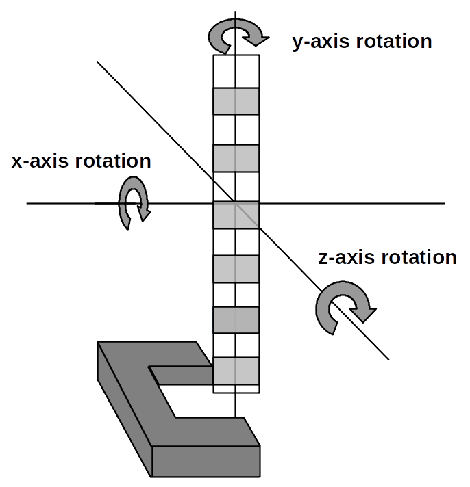
• Systemic errors in angle in dropping the ruler: While we tried to drop the ruler straight, there's always the possibility it was at a slight angle. It could have been rotated slightly about the \(x\), \(y\), or \(z\) axes. For each axis rotation, for each part, how would this affect your final measurement of \(g\) - would you overestimate, underestimate, or neither? Explain your answer.

  

• Systemic Error: Air Resistance: There are multiple models of air resistance of a falling object. A simple one has the force of air resistance being proportional to the cross-sectional area of the object falling.³ Discuss what this implies for the relevance of air resistance as a systemic error in this lab.
• Correlations in D uncertainty: When we propagate error from \(D\) into \(d\), we are implicitly assuming that the measurement uncertainty is more important than the actual variation in width from segment to segment. If the variation in width were far larger, then we should instead be treating our measurement of \(D\) as the sum of the different widths, dividing by \(N\) to give the average of many measurements, and the uncertainty in any particular width would be calculated according to the uncertainty in a "particular measurement." What is the new error propagation if we do this procedure? Based on your looking at the fence we use, is our assumption of the relative size of the two errors justified? (In other language, we are assuming that our errors in measuring the different segments are correlated.²)

Guide to Uncertainty Propagation & Error Analysis (Quick Reference)

PHY133/134 Plotting Tool

Photogate Reference Document

Kinematic Plot Sketching Paper