Oscilloscope
In this lab exercise you will gain a working knowledge of how to use an oscilloscope by measuring the amplitude of a square wave and the frequency of a sine wave.
Note that the goal of this experiment (from a learning perspective) is largely to give you an understanding of this (somewhat complicated) instrument, so that we can use it in future experiments without requiring further explanation.Hoveroverthese!
- 1 Oscilloscope with 1 Banana/BNC Adaptor
- 1 Function Generator with 1 Banana/BNC Adaptor (Koolertron or Juntek brand)
- 2 Banana cables, 1 Alligator Clip
- Record data in this Google Sheets data table
A description of how the oscilloscope works can be found here: Oscilloscope Description
A description of how the function generators work can be found here: Function Generator Description
In short, the oscilloscope is going to measure an abstract quantity (that you'll learn more about later in the course1) which we call "voltage." For now, you can interpret it by its other name, "electrical potential" - literally, it is the "potential for electricity" (as in, put it in a closed circuit and you get electric current).
It measures this "voltage" and plots it as a function of time. This is what appears on the oscilloscope screen.
In more detail: the oscilloscope starts by outputting a dot at the left-hand side of the screen, and moves up and down with the voltage input as it moves to the right. Then, it jumps back to the left, and draws it again. If it moves fast enough (which it will, given how we'll be using it), this will look like a curve as it moves across the screen.
There are some additional (very important) subtleties, but we'll "hide" these complexities in this course, in the sense that you won't be expected to understand them in detail - just follow the instructions for how to set the relevant switches, and things should (hopefully) work.
Click here for more information about these subtleties:
If the oscilloscope really just restarted the moment it reached the end, then it might not have traced out an integer number of waves as it crossed the screen. This means it would start the next trace at a different point on the wave than it started the first trace, and you wouldn't see a coherent trace - just a bunch of sine waves with different phases piled on top of each other.
Accordingly, our instrument has to ensure that it starts at the same point on the wave each time. The way it does this is using what we call a trigger - it only starts a trace when the voltage crosses some fixed (specified) value.
There are a few settings on the oscilloscope that relate to this trigger, with the primary one being the TRIG LEVEL knob. This knob sets the voltage at which it triggers a new wave. If you turn this knob outside the ranges of values that your input actually reaches, you'll just get random chaos (it'll start at random times).
Beyond analyzing periodic signals in a coherent way, this "trigger" feature allows for analysis of much more general signals. For instance, a radioactive decay might appear as a "pulse" on our screen that happens at seemingly random times; the trigger allows us to detect these pulses and overlap them automatically. (Actually, digital instruments can sometimes be better for this, since our oscilloscope can't see anything "before" the trigger - it doesn't "save" that information, even temporarily, unlike a digital scope.)
Later in this course, we'll be analyzing two voltages at once: an "input signal" and a "system response." (An imaginary experiment that illustrates the idea: "if I push with this frequency and amplitude, my system oscillates with this frequency and amplitude.")
Typically, we put our input signal into CH2 and measure a response through CH1. We then want to trigger based on our input channel (since that is more "reliable," in a sense - we know what we should get), so we set SOURCE to CH2 (which says that determines the trigger). The VERT MODE changes which of these we display, with DUAL showing both.
Basic Oscilloscope Setup
Begin by unplugging any red or black cables from the front of all devices, before you turn anything on. (Always a good first step!)
Let's first get the oscilloscope to a good "default" position for getting some basics down:
- Press in the red power button (just to the right of the screen)
- Ensure that all other buttons (the ones below the screen, the "Storage/Analog" button, and the "XY" button) are unpressed (i.e., pushed out).
- Ensure that all knobs that can be pulled out/pushed in, are pushed in.
- Set VAR SWEEP and the two red VAR knobs (on the front of the big white ones) to CAL'D (rightmost position)
- Set HOLDOFF (top-right corner, second knob to the left) to the leftmost position. Set TRIG LEVEL to the center (vertical) position.
- Set COUPLING to AC and SOURCE to CH1. Set the VERT MODE switch to CH1 as well.
- Set the switch on the left-hand side to GND (ground)
- Turn TIME/DIV (the big knob on the bottom right) all the way to the right
- Turn the left POS knob (just to the right of the red power button) until you see a line across your screen.
So, at this point you should just see a steady green line across your oscilloscope. If you can't get this to appear, double-check all your knobs (also try setting your INTENSITY knob all the way to the right), then consult your TA.
Once you have that on your screen, what you are measuring (physically) is just "zero," hence why we get a steady line: voltage isn't changing over time.
Intensity and Focus
The first knobs we will tweak are the two in the upper-right corner of your screen: INTENSITY and FOCUS.
Turn the INTENSITY knob first. As you can see, it makes the screen brighter and dimmer. Usually halfway turned (pointed up) will work here: you want it to be easy to see, but if you set it too bright then your line will be unnecessarily thick, which will increase your uncertainty.
Next, the FOCUS knob. You should see that turning this knob focuses and defocuses your line. You want your line as focused as possible - a narrower line is a more precise measurement!
Whenver you set up your oscilloscope, these should be the first things you check.
Setting Up a Square Wave
Turn the TIME/DIV knob up to 1ms (take note of the units there - the knob has several units to pick from!). Set the left-hand VOLTS/DIV knob to 0.2V.
Clamp an alligator clip onto the little metal clip in the bottom-center of the device (where it says CAL, along with a few numbers).
Wire a banana cable from this spot to the red port of CH1 (the left-hand wire input, which should hopefully already have an adaptor).12
Now, set the left-hand switch from GND to DC. You should now see a nice square wave that we can play with.
Adjusting Positions
Let's begin with the POSITION knobs. If you turn the knob in the upper-right hand corner of the device, the wave will shift left and right. If you turn the POSITION knob corresponding to channel 1 (to the right of the power button), it should move up and down.
This might sound strange: if we can freely move it up and down, how does that result in a "measurement"? We can set it to anything we want!
This is partially true, but usually for this kind of signal, we only care about the variations in voltage, or we know that they average out to zero (like a sine wave). The variations are directly measureable, so that works fine.
Moreover: if we want to measure the voltage on an absolute scale, we can measure zero by flicking the left-hand switch to GND briefly, so we could measure absolutely if we wanted to - perhaps even set GND to the middle of the screen. (In this class, though, we won't ever need to to this - we'll only ever be interested in the variations, for which we won't need to know what "zero" actually is.)
The ability to move stuff around is primarily so you can put it into a nice part of the screen to look at. (For one signal, this might seem esoteric, but when you have two signals on the screen at the same time, it can be useful.)
Adjusting Scales
The other knobs that do "interesting" (i.e., "useful to us") things here are the big gray ones: the VOLTS/DIV and TIME/DIV knobs.
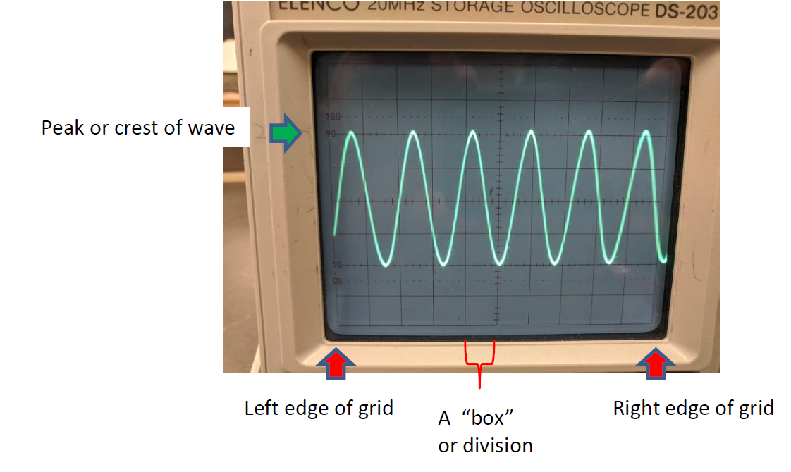
The TIME/DIV knob measures the length of time that one horizontal box describes. (Note: one box, not one tick mark.)
Right now, you should observe that one period of the wave is one box. According to the knob setting we chose, one box is one millisecond. Therefore, the period of the wave is one millisecond.
Since \(f=1/T\), we can calculate the frequency. Since 1/(1ms)=1kHz, the frequency of our square wave is therefore 1kHz.
Look now at the numbers right by the little metal clip we attached the alligator clip to. One of these numbers says "1kHz" - the frequency of this square wave is 1kHz. So it matches what we expect!
Turn the knob by a click or two downwards. Check real quick: does the result still make sense on this new setting?
(Calculate the frequency and see if it is still the expected 1kHz. This isn't to hand in, just to get settled with the idea of the measurement.)
Now, look at the vertical setting: VOLTS/DIV. This is the same idea on a different axis. As our first measurement, we'll check whether the amplitude of the square wave is what we expect.
Part I: Square Wave Amplitude
Adjust the square wave with the POS settings and the VOLTS/DIV setting until your screen is almost entirely filled with a few periods of the square wave. Record the VOLTS/DIV and TIME/DIV on your data sheet for later reference.
On the paper provided, sketch a copy of what you see on the oscilloscope screen.3
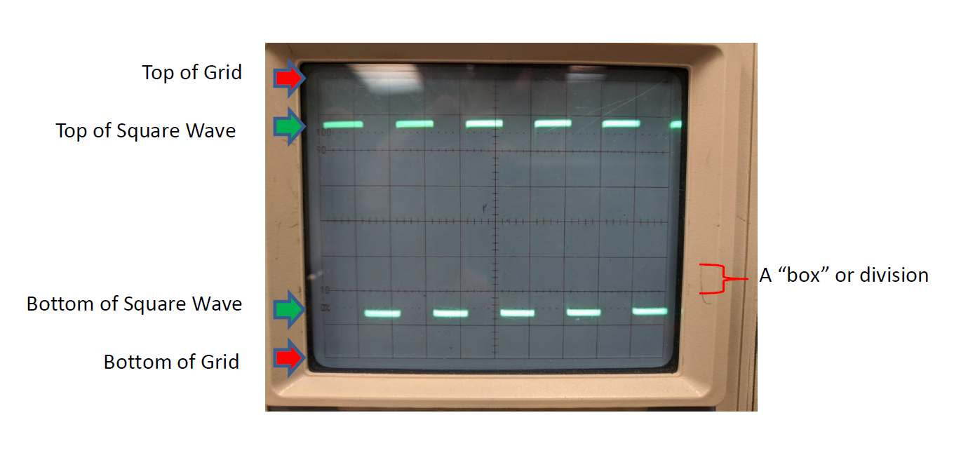
Now: count the number of boxes vertically from the bottom of the grid on the screen to the bottom of the square wave, and record this on your data sheet as your "low reading." 4 (Count the big boxes, not the little tick marks.) Round to the nearest half-tick-mark. Estimate your uncertainty in this reading based on how precise you think your measurement is (generally at least 0.5 tick marks).
Repeat this measurement, except this time counting from the bottom of the grid to the top of the square wave, and record this as your high reading.
Using your VOLTS/DIV, convert these to the physical upper and lower voltages for the square wave. The difference between these will be the "peak-to-peak" amplitude of the square wave.1
We will compare this amplitude to the expected amplitude recorded below the little metal clip on the oscilloscope. Record this expected amplitude on your data sheet.
Part II: Sine Wave Frequency
Start by "un-wiring" your connections for Part I.
Refer to the Reference Guide for Function Generators for this part. You will need to identify what sort of function generator you have in order to know how to use it correctly.
Turn on your function generator and wire it to CH 1 (red to red and black to black).5
Set your function generator to output a sine wave at a frequency of approximately 3kHz.6
If you tweak your position and scale knobs as necessary, you should now be observing a sine wave.
Adjust this sine wave until it takes up most of the screen vertically and you have ~5 periods of the wave on screen. Record the VOLTS/DIV and TIME/DIV on your data sheet for later reference.
Sketch the sine wave you see on the paper provided as you did for the first measurement.7
We'll now measure the time it takes to complete the periods you have on screen. Choose some point on the first oscillation you see to measure from (say, the top of the peak). Count the number of waves between that point and the corresponding point on the last wave on your screen. Record this as the number of waves. (Be careful not to get an off-by-one error!)
Now, record the number of boxes from the left edge of the grid on the screen to the point where you started counting waves as your start reading.8 Similarly, record the number of boxes from the left edge of the grid to the point where you stopped counting waves as your end reading. Note unlike before, we're counting horizontal boxes this time, not vertical boxes.
Understanding Triggering (Optional But Useful)
First, if you have not already, read the supplementary background material about the additional subtleties in the blue collapsible section above. Let's have an intuition as to what this "TRIG LEVEL" does.
Begin set up with the sine wave (per the previous part). Then, turn the horizontal position knob to the right - we want to see where our wave begins (i.e., what voltage the oscilloscope reads when it starts its trace).
Now, adjust your TRIG LEVEL knob up and down a little bit. What happens to the starting point on the wave? What happens when you turn the trigger level up too high (or down to low), above the top (or below the bottom) of the wave?
Finally, set it back to a "reasonable" level, and try "pulling out" that knob. What happens to the starting point now?
Analyzing Two Signals (Optional But Useful)
If you choose to do this part, it will require two function generators or a function generator with two outputs. We will assume that you have a Koolertron or Juntek device with two outputs.
Plug Channel 1 (yellow) of your function generator into CH1 of the oscilloscope. Plug Channel 2 (blue) of the function generator into CH2 (not the rightmost port, the one to the left of that). Set your oscilloscope CH2 settings to the same as CH1 (DC on the lever, same VOLTS/DIV, etc.). Set the VERT MODE switch to DUAL.
Have both channels of your function generator set to the same frequency sine wave (or similar, at least, depending on which type you have). Now, look at your oscilloscope: you should see two sine waves. (If you don't see two signals but did set VERT MODE to DUAL, try adjusting your vertical POS knobs. If one seems to be moving, that's fine.)
Look at both; by adjusting the vertical POS knobs, see which is the CH1 input and which is the CH2 input. (Which one wiggles when you turn each POS knob?)
Now: vary each VOLTS/DIV knob. What does each knob do to each signal? What about TIME/DIV and horizontal position?
Now, set your function generators to similar frequencies (but not exactly the same). What do you observe about the behavior? Which one is "stable" and which one is "moving"? What if you change the SOURCE from CH1 to CH2?
A final thing that's fun (but unrelated to what we'll be doing in the future): press in the X-Y button. This plots the two voltages against each other (time is no longer an axis). What happens when the frequencies are the same? What if they're only similar? What if they're not the same, but one is twice the other? Etc. (These plots are called Lissajous figures.) Feel free to play!
Understanding The Rest (Optional; No Procedure)
A few comments on the other parts of the oscilloscope that we haven't explained:
- HOLD OFF: It is possible to impose a "delay" between when one sweep ends and the next starts (useful if you don't want two signals very close together that may overlap). HOLD OFF controls this delay. We don't want a delay (and having one can lead to an annoying "flickering"), so we set this to the minimum value. (Occasionally, setting HOLD OFF a bit higher than the minimum value - say, a quarter-turn - fixes some problems, such as a flickering "doubled" sine wave.)
- STORAGE/ANALOG: Our oscilloscopes have some fancier features that allow you to "store" an image to the screen (and "save" it for later). This button (and the buttons below the screen) deal with that feature.
- VAR (red knobs) and VAR SWEEP: These change our VOLTS/DIV and TIME/DIV values, respectively. However, if they're not in the rightmost position, we have no idea what the VOLTS/DIV and TIME/DIV actually are. Hence, we always keep them in their rightmost position. (In general, these are used to make "prettier pictures" when the actual values don't matter.)
- EXT TRIG: You can actually have a third input act as a trigger in addition to two signals, and set SOURCE to EXT to use this. We won't do anything so complicated.
- COUPLING: The oscilloscope has an amplifier for the trigger that can be used in more interesting ways, but is mainly useful for repairing CRT televisions.
- AC GND DC: GND grounds the circuit, measuring zero, and DC simply measures the signal. AC puts the signal through a capacitor first, which can be useful for analyzing very fast signals.
Oscilloscope Sketches
In this lab, you will make two oscilloscope sketches. Each of them should have the following:
- A title for the plot.
- Labelled axes, with units: "Voltage (V)" for the y-axis and "Time (s)" for the x-axis (with the units changed if you use mV, ms, or μs instead of V and/or s - choose appropriately for your Volts/Div and Time/Div settings).
- Numbered axes: choose an (arbitrary) origin for your plot, and put numbers on your axes, where the numbers correspond to physical quantities. That means you should use your Volts/Div setting to determine the y values and the Time/Div setting to determine the x values.
- A sketch of the curve that is visible on your screen (of course), drawn to the best of your ability.
You should ignore the little 0/10/90/100 numbers on the left side of the screen: none of those are relevant.
On the Data Sheet
You should show the following calculations, with error propagation for each:
- Part I:
- Convert your vertical "box" measurements into physical voltages.
- Take the difference of your physical voltages to measure the "peak-to-peak" amplitude of the square wave.
- Part II:
- Convert your horizontal "box" measurements into physical times.
- Take the difference of these times to calculate the total time for multiple waves.
- Divide by the number of waves that occur in that time to get the period.
- Take one over the period to get the frequency.
Based on the data you extract in this part, answer the questions in the data table about the compatibility of your results with expectation.
There are no questions for this lab (aside from the ones on the data table).
Guide to Uncertainty Propagation & Error Analysis (Quick Reference)
Hovering over these bubbles will make a footnote pop up. Gray footnotes are citations and links to outside references.
Blue footnotes are discussions of general physics material that would break up the flow of explanation to include directly. These can be important subtleties, advanced material, historical asides, hints for questions, etc.
Yellow footnotes are details about experimental procedure or analysis. These can be reminders about how to use equipment, explanations of how to get good results, troubleshooting tips, or clarifications on details of frequent confusion.
Note that this is different (by a factor of 2) by what we call the "amplitude" of the wave when we study waves in PHY121. "Peak-to-peak" is top-to-bottom, whereas our usual notion of amplitude is top-to-middle. (It's a purely terminological subtlety; peak-to-peak happens to be a more handy measurement in certain circumstances, including this one.)
To read ahead about voltage, see the beginning of KJF Ch. 21. For the purposes of this lab, you can just treat it as an abstract "signal," though.
If your adaptor is in good condition, there should be a red and black terminal. If yours is missing one (or if you get weird results), look for the little "nub" on the side of the adaptor that says "GND" on it - this is on the side that is "black" (hence the other side is "red").
It is good practice, but not necessary, to also wire a black wire from the black terminal of Cha 1 to the GND input next to the little metal clip on the oscilloscope. This is not necessary because Cha 1 and the little metal clip already share the same "signal common", provided by the oscilloscope.
Remember everything you need to make a good plot, which is not just the signal on the screen! For more detail, see the analysis section, below.
If it has multiple ports, see the document to determine what port is the correct one to connect. Ideally, the correct port will have the adaptor (for our cables) already on it.
Again: see the instructions linked above to determine how to do this, because all of the function generators work slightly differently here.
Again: see analysis section below; make sure your sketch has all the appropriate accoutrements.