In this lab, you will be plotting out the electric field of two different charge configurations: a set of parallel plates and a dipole.

You will plot out the potential at different positions on a carbon sheet. This will allow you to pick out equipotentials, from which you can sketch the field lines.^{Hoveroverthese!}

• 1 Hantek PC-Based Digital oscilloscope with BNC to banana adapter
• 2 Voltage Probes (one stationary, one hand probe)
• 1 Platform
• 2 Carbon Acetate Sheets (one parallel plate, one dipole)
• 1 Power Supply
• 1 Meter Stick
• 4 Banana Cables
• Use this Excel template to make 3D and contour plots
• Record data in this Google Sheets data table

Electric Field & Voltage

This lab explores the relationship between electric field strength, voltage, electric field lines, and equipotentials.¹

The electric field \(\vec{E}\) is a vector field, meaning it is a vector associated with every point in space. The closely related quantity of voltage \(V\) is a scalar function of position, and is related to electric field.

Take two nearby points in space, \(\vec{x}_1\) and \(\vec{x}_2\), and suppose the voltages at these points are \(V_1=V(x_1)\) and \(V_2=V(x_2)\). With these voltages, we can approximately¹ compute the component of electric field in the \(\vec{x}_2-\vec{x}_1\) direction as:

$$E_{\vec{x}_2-\vec{x}_1\text{ component}}=-\frac{V_2-V_1}{|\vec{x}_2-\vec{x}_1|}\label{EFieldStrength}$$

Field Lines & Equipotentials

While an explicit calculation of electric field is excellent, we are often more concerned about getting a picture of electric field than getting an exact description. A good tool to get this qualitative picture is electric field lines.

Electric field lines start at positive charges (or somewhere infinitely far away) and end at negative charges (or somewhere infinitely far away). In between, they always travel parallel to the electric field. They never cross or make loops.²

Once we have these field lines, we can interpret them to get a qualitative understanding of field strength: "bunching" of electric field lines (i.e., where they get dense) indicates that the electric field is stronger there, and "spreading" indicates that the electric field is weaker.

A different part of our qualitative picture is the equipotential lines. These are lines (or, in 3D, planes) on which the voltage is constant. If we space our equipotentials by some fixed voltage intervals (e.g., put an equipotential every 1V), then we can use equation \eqref{EFieldStrength} to show that "closer together" equipotentials mean stronger fields (because \(V_2-V_1\) is the same, but \(|\vec{x}_2-\vec{x}_1|\) decreases.)

Also from equation \eqref{EFieldStrength}, by considering two "nearby" points, we can show that the component of electric field parallel to the equipotential is zero; hence, the electric field is perpendicular to equipotentials. This allows us to make the key relationship between equipotentials and field lines: equipotentials are always perpendicular to electric field lines.

This allows us to understand the qualitative behavior of our electric field lines (and hence our electric field) from our equipotentials, which can be determined by simply measuring voltage. That is what we will be doing in this lab.

To measure voltage, we are going to use a device known as a voltmeter. This device measures the voltage between its endpoints.³

Physics Behind Electric Fields

Electric fields are made by charges. For a single isolated charge \(q\), the electric field is given by Coulomb's law, with strength:

$$|\vec{E}|=\frac{k|q|}{r^2}$$

Here, \(k=8.99\times 10^9\frac{\text{Nm}^2}{\text{C}^2}\) is Coulomb's constant and \(r\) is the distance between the charge and the point you are measuring.

If you have multiple charges, you add together their electric fields (with the \(r\) modified appropriately for each charge!) to get the total electric field. This suffices for electric fields made by pointlike charges; for electric fields made by "diffuse" charges (spread out over some region), the same idea holds, but the math gets more complicated.

One key configuration of charges is one or more "plates" (infinite planes) of charge. Each plate makes an electric field that is constant in strength, emitted directly outward or inward (depending on the sign of the charge on the plate). The strength of the electric field depends on the charge density (charge per unit area) of the plate.

Similar to point charges, if there are multiple plates, we add together their electric fields to get the overall electric field. (Same if there is a plate and point charges, or any other combination of chrage configurations.)

Going beyond charges themselves, one of the key electrical objects we use is a conductor. These materials (usually metals) allow electrons to move around freely (contrasted with insulators) whenever there is an electric field.

After a short time, a conductor's electrons will have rearranged themselves so that the electric fields inside are zero. This means that the entire conductor is a solid equipotential; the voltage is constant everywhere within it.

Ultimately, all of the net charge ends up on the edge of the conductor, and thus field lines end there. The field lines at the edge of a conductor also always enter the conductor perpendicularly, because the conductor is an equipotential.

Part I: Setup

First, place the carbon sheet with the "parallel plates" configuration (the one that looks like a pair of "T" shapes) on the platform. Place the clamps such that they are contacting the silver conductive strips coming out the back of the plates.

Wire a red wire from the red terminal of the power supply to the end of the platform with the higher row numbers.¹ Wire a black wire from the black terminal of the power supply to the other end of the platform.

Get the oscilloscope device and pc software running. There will be a BNC to banana adapter on Channel 1 of the osciloscope.

Wire a black wire from the black (-) port of Channel 1 on the oscilloscope to the stationary probe (the one with the stand). Wire a red wire from the red (+) port of Channel 1 to the hand probe (the one with the handle).

Plug in the power supply, turn it on, and set it to 7.5V.

Place the stationary probe on the silver conductive surface that is connected to the black port on the power supply. For optimal results, place it at the base of the "T" (the edge closest to the black probe).

Place your other probe on the other silver conductive surface (anywhere, doesn't matter). The oscilloscope will now have a (roughly) flat signal which is approximately +7.5V (or a bit less) when you do so. If you see -7.5V, you have one of your sets of wires the wrong way around.

Part IIA: Parallel Plate Map

Open Excel on either your own personal computer or on one of the lab computers. Open this template.²³

Leaving your stationary probe where we put it in Part I, place your hand probe on each other point on the sheet. Record the voltage, as measured on the oscilloscope, in the corresponding cell on your sheet. (Yes, this will take a while, since we're measuring 221 voltages... twice.)

You should observe a relatively smooth gradient going from the high voltage plate (~7.5V) to the low voltage plate (0V). If a single data point looks strange (much higher or lower than nearby points), you probably either made a typo or have a poor contact at that point.⁴

Check the other two tabs on that document. One of them contains a 3D plot, and the other contains a contour plot. Look at your 3D plot, and ensure it looks smooth-ish. If not, identify the points where it is not, and double-check them.

If you are working on the lab computers, send yourself a copy of your data sheet (ideally, both as a .xlsx file and as a .pdf file).

Part IIB: Parallel Plate Plot

We are now going to take this data and show that our electric field is (approximately) constant between these plates.⁴

Take a sequence of voltage measurements that proceed from one plate to the other (not including the voltages on the plates themselves, or behind them), and record them on the data sheet (the Google Sheets one, not the Excel 3D Plot one). Take an appropriate uncertainty (last decimal place displayed on the voltmeter).

Then, for each voltage point, measure the "position" of that dot on your carbon sheet as the distance between the dot and the near edge of the low-voltage plate, and estimate uncertainty.

Part IIIA: Dipole Map

Connect the dipole sheet to the terminals as you did the parallel plate sheet previously (same orientation). Leave your wiring the same, and check that you record 7.5V(-ish) as before.

Download another copy of the template (or, if you've sent yourself a copy of the results already, delete the data you have in there) and fill it out in the same way for the new configuration.

Again, check that the picture you observe matches what you expect before moving on.

Part IIIB: Dipole Calculations

Now we are going to attempt to compute the charge on each pole. We will take two nearby voltages and use them to compute electric field at that point, then use that electric field and Coulomb's law to compute the charge on the pole. The following picture illustrates this process (both the idealized picture and what our measurements actually look like):

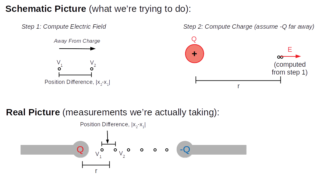
Note we'll do this for each of the two charges. Now, for more concrete instructions on how to do this.

Take the high-voltage pole of your dipole. On your data sheet, record the voltages in two consecutive points going off to one side - e.g., at the points (7,10) and (6,10), with uncertainty.

Record the difference in position between these two points (as you measure), with uncertainty, as illustrated on the above diagram. Also record the distance between the "halfway point" between these two points and the center of the high-voltage pole as \(r\) (with uncertainty), again as illustrated above.

Repeat these measurements for the low-voltage pole (measure distance from that pole, the two closest voltages, etc.).

Qualitative Results

First, look carefully at the 3D and contour plots made by Excel, and think carefully about what they mean and how to interpret them. (Your contour plot is directly showing you some equipotentials: where and how, and corresponding to what voltages?)

Then, for each charge configuration, print out the paper picture corresponding to that configuration: Parallel Plate and Dipole. Then, on that printout,⁵ based on the plots you got from Excel, do the following:⁶

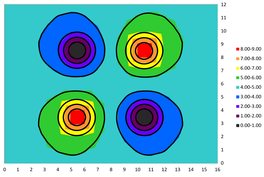
• Sketch the equipotential lines. (You can "smooth" them compared to what Excel gives you.) As an illustration, here's a plot made with a charge configuration we did not do in this lab (a quadrapole):

  

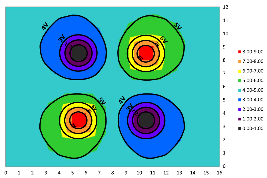
• Mark down the voltage that each contour corresponds to. [You can tell this based on what it's the boundary of; e.g.: the line between the "5-6V" region and the "6-7V" region must be at 6V.] Your results should now look like this (except with your configurations):

  

• Sketch out the electric field lines. Include the direction the field lines point (from high to low). As an example:

  

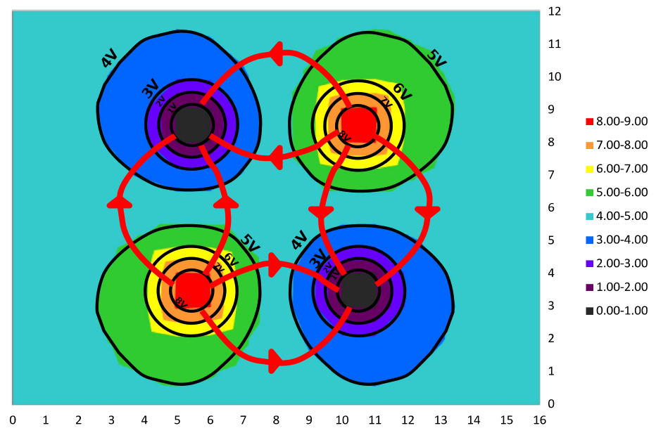
• Dipole only: Circle the region(s) of the sketch where the electric field is the strongest.

In addition, make a plot of voltage vs. position for your parallel plate measurements (with all appropriate plot accoutrements).

Then, write a discussion of your results that covers the following points:

• What do the field lines do in the "parallel plates" configuration in the center of the two plates? What does this show? What about at the edges of the two plates?
• In the dipole configuration, what is the shape of the lines? How do you know where the field is the strongest?
• Is your plot of voltage vs. position linear? What does that tell you? What does the slope tell you?

Calculating Charges

We will now use Coulomb's law to calculate the charges we were dealing with in the dipole.

For each set of measurements you took in part IIIB, do the following:

• Calculate the difference between the voltages, and propagate uncertainty.
• Calculate the "average" (component of) electric field using formula \eqref{EFieldStrength}, and propagate uncertainty.
• Assume this electric field was measured at the "average position" described by \(r\). Using Coulomb's law, calculate the charge \(q\). Be sure to have the appropriate sign on these charges!

Note: in this last step, you can assume only the "close" charge matters. The "far" charge (the negative charge for your high-voltage measurements and vice-versa) will be contributing little enough electric field that we will neglect it.

Finally, compare your positive and negative charges, and answer the question on the data table.

Your TA will ask you to answer some of the following questions (they will tell you which ones to answer):

Experimental Questions:

1. We expect a conductor to be a constant voltage throughout. The conductive surface (silver marks) is mostly a constant voltage, but sometimes you may observe a millivolts-ish difference between different points on it. What does this mean about said conductive surface?
2. What errors could have impacted the qualitative behavior (i.e., the shape) of our electric field lines? (Hint: what makes electric fields? How could such things have been present in the ambient environment?) [Note: we're looking for things that could have impacted our actual, physical field lines here, not just altered our measurement of them.]

Theoretical Questions:

1. Suppose you swapped positive and negative charges in the dipole arrangement. What would happen to the electric field lines (both shape and direction)? Would they be the same or different, and if different, how so?
2. Suppose you made both charges from the dipole configuration positive, or both negative. Would the electric field line configuration be the same or different, and if different, how so?

For Further Thought:

1. We call the first configuration a "parallel plates" arrangement, but technically, they're not "plates," because they don't extend vertically. Thus, we can more accurately picture this as two lines of charge. Draw a picture displaying what the field lines would be (in 3D) for these "lines" of charge. What does this imply about the "expected" field strength of this configuration in between the lines?⁵

Guide to Uncertainty Propagation & Error Analysis (Quick Reference)

3D Plots Template

PHY121/122 Plotting Tool

Parallel Plates Sketch Paper   Dipole Sketch Paper